Longitudinal Model-Based Meta-Analysis (MBMA) with Monolix Suite

Download data set only | Download all Monolix&Simulx project files V2021R2 | Download all Monolix&Simulx project files V2023R1

In this case study we demonstrate how to implement and analyze a longitudinal MBMA model with Monolix and Simulx.

Introduction
Background
- Canakinumab, a drug candidate for rheumatoid arthritis
- MBMA concepts
Data selection, extraction and visualization
Longitudinal mixed effect model description
Set up of the model in Monolix
Model development: Parameter estimation, model diagnosis, alternate model, covariate search, and final model
Simulations for decision support
- Comparison of Canaki efficacy with drugs on the market
Conclusion
Guidelines for implementing your own MBMA model

Introduction

Due to the high costs of drug development, it is crucial to determine as soon as possible during the drug development process if the new drug candidate has a reasonable chance of showing clinical benefit compared to the other compounds already on the market. To help the decision makers in go/no-go decisions, model-based meta-analysis (MBMA) has been proposed. MBMA consists in using published aggregate data from many studies to develop a model and support the decision process. Note that individual data are usually not available as only mean responses over entire treatment arms are reported in publications.

Because in an MBMA approach one considers studies instead of individuals, the formulation of the problem as a mixed effect model differs slightly from the typical PK/PD formulation. In this case study, we present how MBMA models can be implemented, analyzed and used for decision support in Monolix and Simulx.

As an example, we focus on longitudinal data of the clinical efficacy of drugs for rheumatoid arthritis (RA). The goal is to evaluate the efficacy of a drug in development (phase II) in comparison to two drugs already on the market. This case study is strongly inspired by the following publication:

Demin, I., Hamrén, B., Luttringer, O., Pillai, G., & Jung, T. (2012). Longitudinal model-based meta-analysis in rheumatoid arthritis: an application toward model-based drug development. Clinical Pharmacology and Therapeutics, 92(3), 352–9.

Canakinumab, a drug candidate for rheumatoid arthritis

Rheumatoid arthritis (RA) is a complex auto-immune disease, characterized by swollen and painful joints. It affects around 1% of the population and evolves slowly (the symptoms come up over months). Patients are usually first treated with traditional disease-modifying anti-rheumatic drugs, the most common being methotrexate (MTX). If the improvement is too limited, patients can be treated with biologic drugs in addition to the MTX treatment. Although biologic drugs have an improved efficacy, remission is not complete in all patients. To address this unmet clinical need, a new drug candidate, Canakinumab (abbreviated Canaki), has been developed at Novartis. After a successful proof-of-concept study, a 12-week, multicenter, randomized, double-blind, placebo-controlled, parallel-group, dose-finding phase IIB study with Canaki+MTX was conducted in patients with active RA despite stable treatment with MTX. In the study, Canaki+MTX was shown to be superior to MTX alone.

We would like to compare the expected efficacy of Canaki with the efficacy of two other biologics already on the market, Adalimumab (abbreviated Adali) and Abatacept (abbreviated Abata). Several studies involving Adali and Abata have been published in the past (see list below). A typical endpoint in those studies is the ACR20, i.e the percentage of patients achieving 20% improvement. We focus in particular on longitudinal ACR20 data, measured at several time points after initiation of the treatment, and we would like to use a mixed effect model to describe this data.

MBMA concepts

The formulation of longitudinal mixed effect models for study-level data differs from longitudinal mixed effect models for individual-level data. As detailed in

Ahn, J. E., & French, J. L. (2010). Longitudinal aggregate data model-based meta-analysis with NONMEM: Approaches to handling within treatment arm correlation. Journal of Pharmacokinetics and Pharmacodynamics, 37(2), 179–201.

to obtain the study-level model equations, one can write a non-linear mixed effect model for each individual (including inter-individual variability) and derive the study-level model by taking the mean response in each treatment group, i.e the average of the individual responses. In the simplistic case of linear models, the study-level model can be rewritten such that a between-study variability (BSV), a between-treatment arm variability (BTAV) and a residual error appear. Importantly, in this formulation, the residual error and the between treatment arm variability are weighted by $\sqrt{N_{ik}}$ with $N_{ik}$the number of individuals in treatment arm k of study i. If the model is not linear, a study-level model cannot be easily derived from the individual-level model. Nevertheless, one usually makes the approximation that the study-level model can also be described using between-study variability, between-treatment arm variability and a residual error term.

This result can be understood in the following way: when considering studies which represent aggregated data, the between-study variability represents the fact that the inclusion criteria vary from study to study, thus leading to patient groups with slightly different mean characteristics from study to study. This aspect is independent of the number of individuals recruited. On the opposite, the between-treatment arm variability represents the fact that when the recruited patients are split in two or more arms, the characteristics of the arms will not be perfectly the same, because there is a finite number of individuals in each arm. The larger the arms are, the smaller the difference between the mean characteristics of the arms is, because one averages over a larger number. This is why the between-treatment arm variability is weighted by $\sqrt{N_{ik}}$. For the residual error, the reasoning is the same: as the individual-level residual error is averaged over a larger number of individuals, the study-level residual error decreases.

The study-level model can thus be written in a way similar to the individual-level model, except that we consider between-study variability and between-treatment arm variability instead of inter-individual variability and inter-occasion variability. And in addition, the residual error and the between treatment arm variability are weighted by $\sqrt{N_{ik}}$.

Before proposing a model for rheumatoid arthritis, let us first have a closer look at the data.

Data selection, extraction and visualization

Data selection

To compare Canaki to Adali and Abata, we have searched for published studies involving these two drugs. Reusing the literature search presented in Demin et al., we have selected only studies with inclusion criteria similar to the Canaki study, in particular: approved dosing regimens, and patients having an inadequate response to MTX. Compared to the Demin et al. paper, we have included two additional studies published later on. In all selected studies, the compared treatments are MTX+placebo and MTX+biologic drug.

The full list of used publications is:

Data extraction

Using an online data digitizer application, we have extracted the longitudinal ACR20 data of the 9 selected publications. The information is recorded in a data file, together with additional information about the studies. The in house individual Canaki data from the phase II trial is averaged over the treatments arms to be comparable to the literature aggregate data. Below is a screenshot of the data file, and a description of the columns.

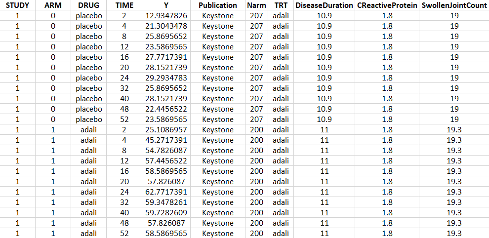
STUDY: index of the study/publication. (Equivalent to the ID column)
ARM: 0 for placebo arm (i.e MTX+placebo treatment), and 1 for biologic drug arm (MTX+biologic drug)
DRUG: name of the drug administrated in the arm (placebo, adali, abata or canaki)
TIME: time since beginning of the treatment, in weeks
Y: ACR20, percentage of persons on the study having an at least 20% improvement of their symptoms
Publication: first author of the publication from which the data has been extracted
Narm: number of individuals in the arm
TRT: treatment studied in the study
DiseaseDuration: mean disease duration (in years) in the arm at the beginning of the study
CReactiveProtein: mean C-reactive protein level (in mg/dL)
SwollenJointCount: mean number of swollen joints

Data visualization

Monolix contains an integrated data visualization module, which is very useful to gain a better overview of the data after importing it. After having open Monolix, we click on New project and then in the Data file option we click on Browse to select the data file. The data set columns are assigned in the following way:

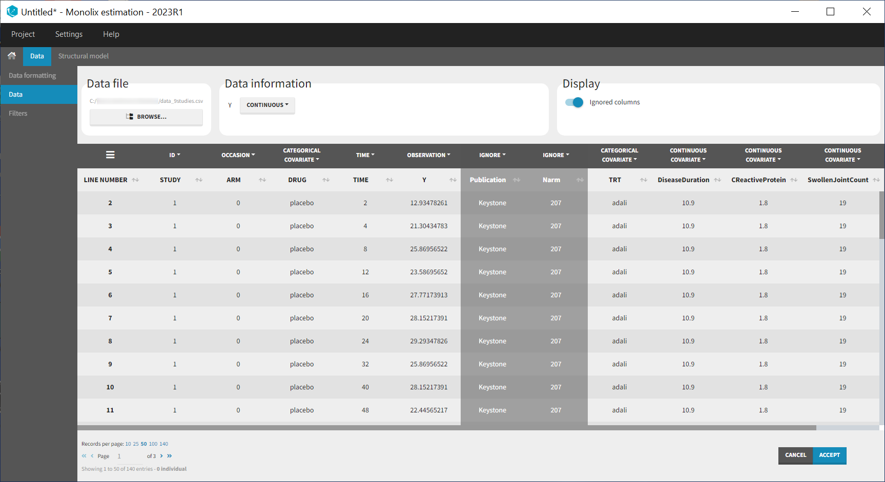
Note that the STUDY column is tagged as ID and the ARM column as OCCASION as we will use the inter-individual and inter-occasion variability concepts of the MonolixSuite to define between-study and between-treatment arm variability instead. All columns that may be used to stratify/color the plots must be tagged as either continuous or categorical covariate, even if these columns will not be used in the model.

After having clicked ACCEPT and NEXT the data appears in the Plots tab. To better distinguish the treatments and arms, we go to the STRATIFY tab and allocate the DRUG and TRT covariates. We then choose to split by TRT and color by DRUG. We also arrange the layout in a single line. In the X-AXIS section of the SETTINGS tab we apply the toggle for custom limits, which automatically sets the limits to 1 and 52.14. In the figure below, arms with biologic drug treatment appear in color (abata in blue, adali in red, canaki in green; customized color selection), while placebo arms appear in black. Note that even in the “placebo” arms the ACR20 improves over time, due to the MTX treatment. In addition, we clearly see that the treatment MTX+biologic drug has a better efficacy compared to MTX+placebo. For Canaki, which is the in house drug in development, only one study is available, the phase II trial.

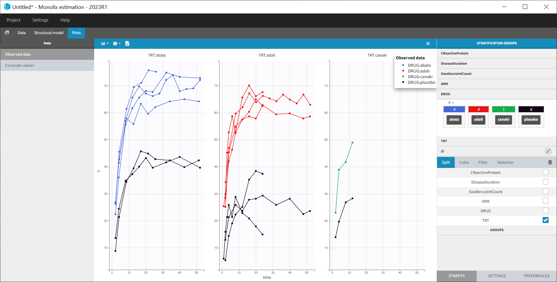
Given this data, does Canaki have a chance to be more effective than Adali and Abata? To answer this question, we develop a longitudinal mixed effect model.

Longitudinal mixed effect model description

Given the shape of the ACR20 over time, we propose an Emax structural model:

$$f(t)= \textrm{Emax}\frac{t}{t+\textrm{T50}}$$

Remember that the ACR20 is a fraction of responders, it is thus in the range 0-1 (or 0-100 if considering the corresponding percentage). In order to keep the model observations also in the range 0-1, we use a logit transformation for the observations $y_{ijk}$:

$$\textrm{logit}(y_{ijk})=\textrm{logit}(\textrm{Emax}_{ik}\frac{t_j}{t_j+\textrm{T50}_{ik}})+\epsilon_{ijk}$$

with i the index over studies, j the index over time, and k the index over the treatment arms. $\epsilon_{ijk}$ is the residual error, it is distributed according to

$$\epsilon_{ijk}\sim \mathcal{N}\left( 0,\frac{\sigma^2}{N_{ik}}\right)$$

with $N_{ik}$ the number of individuals in treatment arm k of study i. Because our data is quite scarce and our interest is mainly on the Emax (efficacy), we choose to consider between-study variability (BSV) and between treatment arm variability (BTAV) for Emax only. For Emax parameter distribution, we select a logit distribution to keep its values between 0 and 1. We thus have:

$$\textrm{logit}(\textrm{Emax}_{ik})=\textrm{logit}(\textrm{Emaxpop}_{d})+\eta^{(0)}_{\textrm{E},i}+\eta^{(1)}_{\textrm{E},ik}$$

$\eta^{(0)}_{\textrm{E},i}$ represents the BSV and $\eta^{(1)}_{\textrm{E},ik}$ represents the BTAV.

For T50, we select a log-normal distribution and no random-effects:

$$\textrm{log}(\textrm{T50}_{ik})=\textrm{log}(\textrm{T50pop}_{d})$$

with Emaxpop_d and T50pop_d the typical population parameters, that depend on the administrated drug d. The BSV (index (0)) and BTAV (index (1)) terms for Emax have the following distributions:

$$\eta^{(0)}_{\textrm{E},i}\sim\mathcal{N}\left( 0,\omega_E^2\right) \quad \eta^{(1)}_{\textrm{E},ik}\sim\mathcal{N}\left( 0,\frac{\gamma_E^2}{N_{ik}}\right)$$

Note that the between-treatment arm variability and residual error are weighted by the number of individuals per arm, while the between-study variability is not, as explained in the section “MBMA concepts” above.

In the next section, we describe how to implement this model in Monolix.

Set up of the model in Monolix

For the error model

In Monolix, it is only possible to choose the error model among a pre-defined list. This does not allow to have a residual error model weighted by the square root of the number of individuals. We will thus transform both the ACR20 observations of the data set and the model prediction in the following way, and use a constant error model. Indeed we can rewrite:

$$\begin{array}{ccl}\textrm{logit}(y_{ijk})=\textrm{logit}(f(t_j,\textrm{Emax}_{ik},\textrm{T50}_{ik}))+\epsilon_{ijk} & \Longleftrightarrow & \textrm{logit}(y_{ijk})=\textrm{logit}(f(t_j,\textrm{Emax}_{ik},\textrm{T50}_{ik}))+\frac{\tilde{\epsilon}_{ijk}}{\sqrt{N_{ik}}} \\ & \Longleftrightarrow & \sqrt{N_{ik}} \times \textrm{logit}(y_{ijk})=\sqrt{N_{ik}} \times \textrm{logit}(f(t_j,\textrm{Emax}_{ik},\textrm{T50}_{ik}))+\tilde{\epsilon}_{ijk} \\ &\Longleftrightarrow& \textrm{transY}_{ijk}=\textrm{transf}(t_j,\textrm{Emax}_{ik},\textrm{T50}_{ik}))+\tilde{\epsilon}_{ijk} \end{array} $$

with

$\tilde{\epsilon}_{ijk}$ a constant (unweighted) residual error term,
$\textrm{transY}_{ijk}=\sqrt{N_{ik}} \times \textrm{logit}(y_{ijk})$ the transformed data,
$\textrm{transf}(t_j,\textrm{Emax}_{ik},\textrm{T50}_{ik}))=\sqrt{N_{ik}} \times \textrm{logit}(f(t_j,\textrm{Emax}_{ik},\textrm{T50}_{ik}))$ the transformed model prediction.

This data transformation is added to the data set, in the column transY.

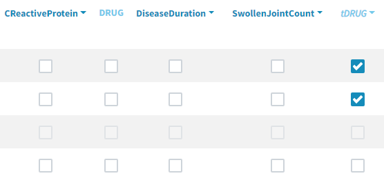
At this stage, we can load the new dataset with the transY column into Monolix and assign the columns as before, except that we now use the column transY as OBSERVATION. STUDY is tagged as ID, ARM as OCCASION, DRUG as CATEGORICAL COVARIATE, TIME as TIME, transY as OBSERVATION, Narm as REGRESSOR, TRT as CATEGORICAL COVARIATE and DiseaseDuration, CReactiveProtein and SwollenJointCount as CONTINUOUS COVARIATE.

To match the observation transformation in the data set, we will have in the Mlxtran model file:

ACR20 = ...
pred = logit(ACR20)*sqrt(Narm)
OUTPUT:
output = pred

In order to be available in the model, the data set column Narm must be tagged as regressor, and passed as argument in the input list:

[LONGITUDINAL]
input = {..., Narm}
Narm = {use=regressor}

In our example the number of individuals per arm (Narm) is constant over time. In case of dropouts or non uniform trials, Narm may vary over time. This will be taken into account in Monolix as, by definition, regressors can change over time.

For the parameter distribution

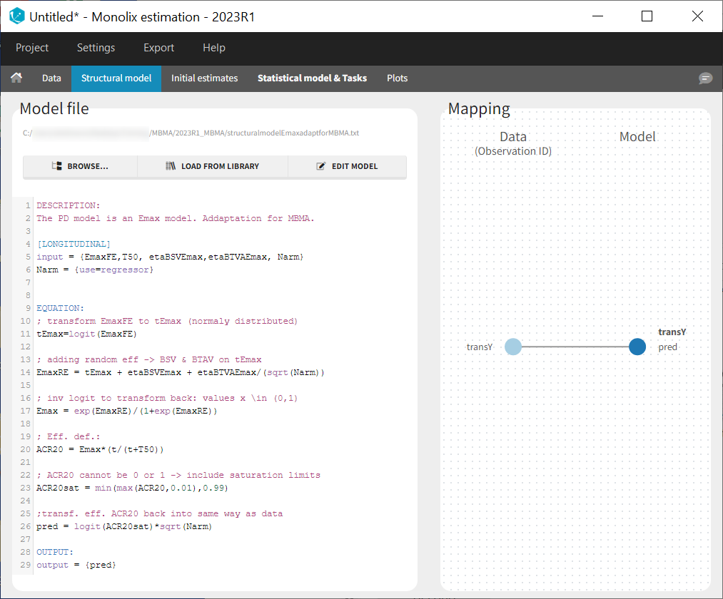
Similarly to the error model, it is not possible to weight the BTAV directly via the Monolix GUI. As an alternative, we can define separately the fixed effect (EmaxFE), the BSV random effect (etaBSVEmax) and the BTAV random effect (etaBTAVEmax) in the GUI and reconstruct the parameter value within the model file. Because we have defined Narm as a regressor, we can use it to weight the BTAV terms. We also need to be careful about adding the random effects on the normally distributed transformed parameters. Here is the syntax for the structural model:

[LONGITUDINAL]
input = {EmaxFE, T50, etaBSVEmax, etaBTAVEmax, Narm}
Narm = {use=regressor}

EQUATION:
; transform the Emax fixed effect (EmaxFE) to tEmax (normally distributed) 
tEmax = logit(EmaxFE)

; adding the random effects (RE) due to between-study variability and 
; between arm variability, on the transformed parameters 
tEmaxRE = tEmax + etaBSVEmax + etaBTAVEmax/sqrt(Narm)

; transforming back to have EmaxRE with logit distribution (values between 0 and 1)
Emax = exp(tEmaxRE)/(1+exp(tEmaxRE))

; defining the effect
ACR20 = Emax * (t / (T50 + t))

; adding a saturation to avoid taking logit(0) (undefined) when t=0
ACR20sat = min(max(ACR20,0.01),0.99)

; transforming the effect ACR20 in the same way as the data
pred = logit(ACR20sat)*sqrt(Narm)

OUTPUT:
output = pred

In addition to the steps already explained, we add a saturation ACR20sat=min(max(ACR20,0.01),0.99) to avoid having ACR20=0 when t=0, which would result in pred=logit(0) (which is undefined).

In the structural model tab, we click on New model, copy-paste the code above and save the model. The model appears below:

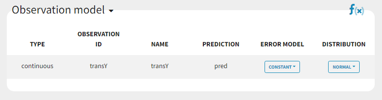
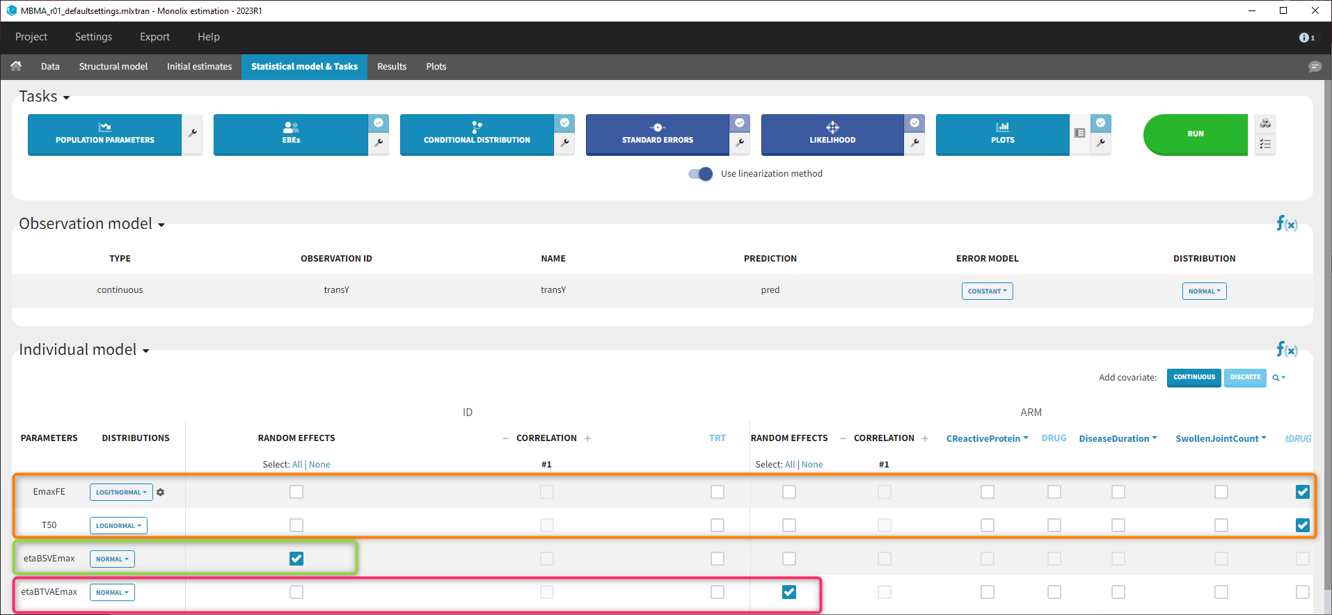
In the next tab Statistical model & Tasks, we will define the statistical part of the model. For the observation model, we choose constant from the list, according to the data transformation done.

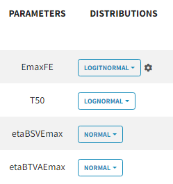
For the parameter distributions, we choose a logit distribution for EmaxFE with distribution limits between 0 and 1 (note that the default iniitla value for EmaxFE is 1 leading to default logit limits (0,1). So the initial value for EmaxFE needs to be changed first, before logit(0,1) can be set), lognormal for T50, and a normal distribution for the random effects etaBSVEmax, and etaBTAVEmax.

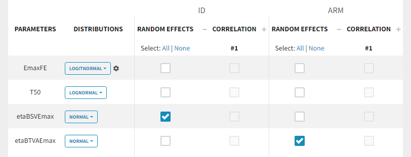
Because with this model formulation EmaxFE represents only the fixed effects, we need to disable the random effects for this parameter, as well as for T50. etaBTAVEmax is equivalent to inter-occasion variability, we thus disable the random effects at the STUDY level (shown as “ID” in the GUI) but enable them at the ARM level. The random effects at both levels are thus set in the following way:

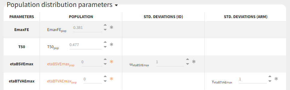
For etaBSVEmax, its distribution is $ \mathcal{N}(0,\omega^2) $ , we thus need to enforce its mean to be zero. This is done in the initial estimates tab, using the cog-wheel button to fix etaBSVEmax_pop to 0. We also do the same for etaBTAVEmax_pop.

For the covariates

As a final step, we need to add DRUG as a covariate on EmaxFE and T50, in order to estimate one EmaxFE and one T50 value for each treatment (placebo, adali, abata, and canaki). Before adding the DRUG column as covariate, we click on the add covariate / discrete button and create a new covariate called tDRUG for which placebo is the reference category:

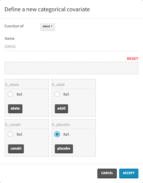
The newly created tDRUG is added on EmaxDE and T50. The other possible covariates will be investigated later on.

Summary view

After this model set up, the Statistical model | Tasks tab is:

Model development

Parameter estimation

Finding initial values

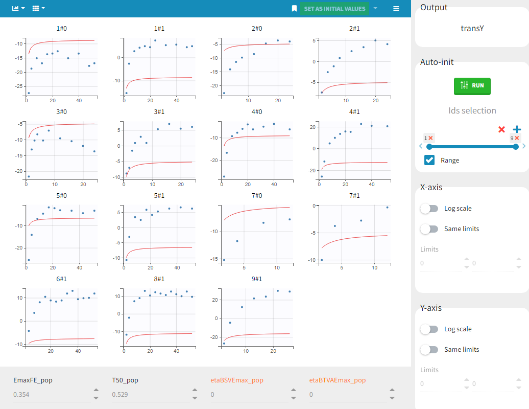
Before starting the parameter estimation, we first try to find reasonable initial values. In the Initial estimates tab, Check initial estimates window, we can either set the initial values of the population parameters by hand, or run the auto-init function that finds the initial values for us, as in the image below. The red curve corresponds to the prediction with the estimated initial values, the blue dots correspond to the transY data.

Choosing the settings

We then launch the parameter estimation task. After around 110 iterations, the SAEM exploratory phase switches to the second phase, due to the automatic stopping criteria.

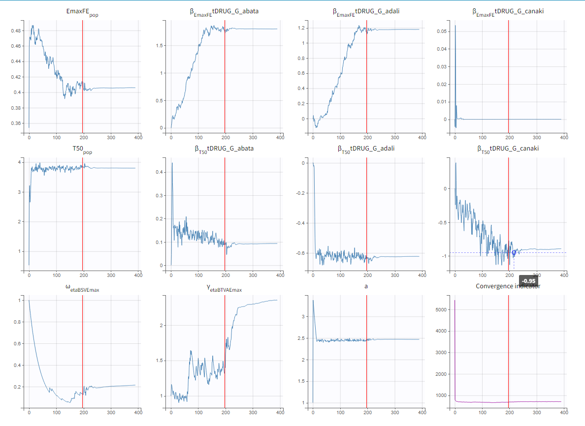
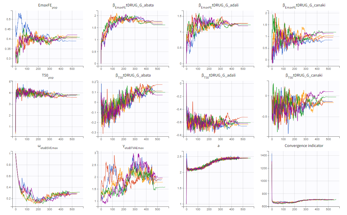
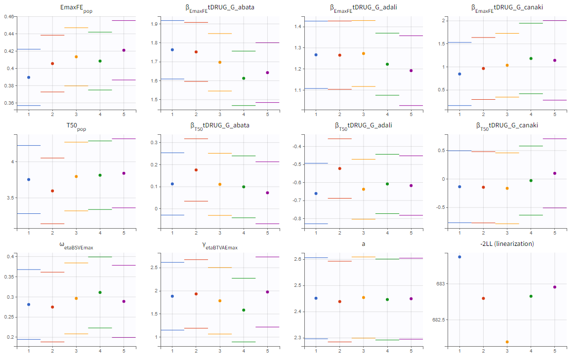
To assess the convergence, we can run the parameter estimation from different initial values and with a different random number sequence. To do so, we click on the “assessment” button and select “all” for the sensitivity on initial values. 5 estimations run will be done using automatically drawn initial values.

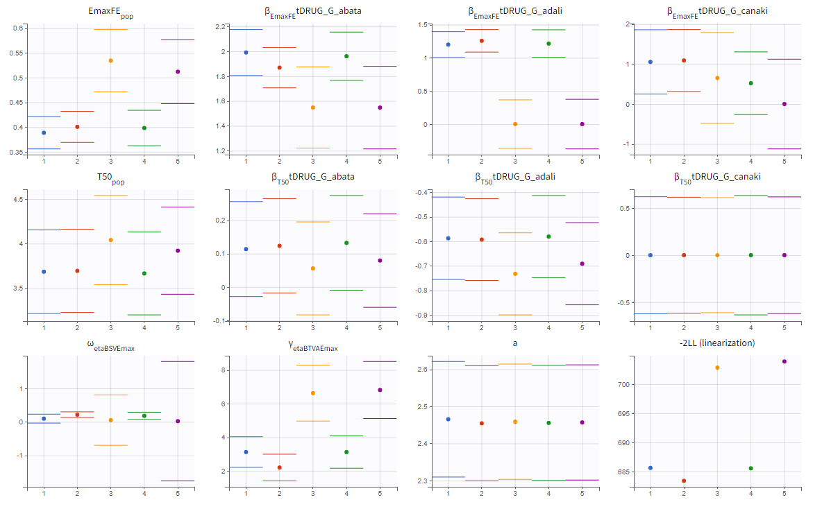
The colored lines in the upper plot above show the parameter estimates trajectories, while the colored horizontal lines in the lower plot above show the standard deviation of the estimated value of each run. We see that the trajectories of many parameters vary a lot from run to run. Parameters without variability, such as EmaxFE, are usually harder to estimate. Indeed, parameters with and without variability are not estimated in the same way. The SAEM algorithm requires to draw parameter values from their marginal distribution, which exists only for parameters with variability.

Several methods can be used to estimate the parameters without variability. By default, these parameters are optimized using the Nelder-Mead simplex algorithm. As the performance of this method seems insufficient in our case, we will try another method. In the SAEM settings (wrench icon next to the task “pop param” in the main window),

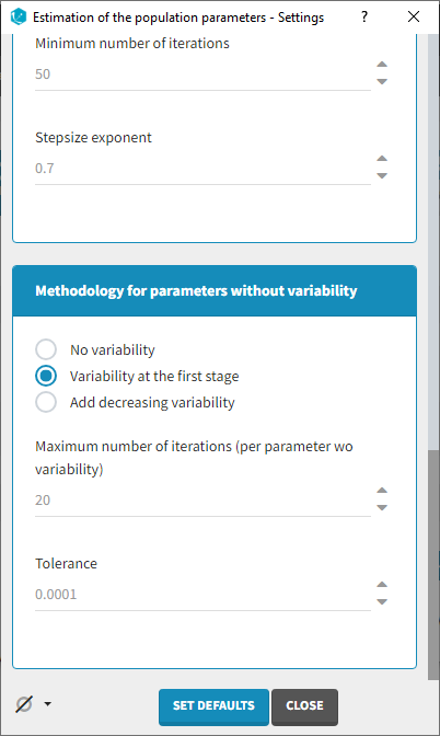
3 options are available in the “Methodology for parameters without variability” section:

No variability (default): optimization via Nelder-Mead simplex algorithm
Add decreasing variability: an artificial variability is added for these parameters, allowing estimation via SAEM. The variability is progressively forced to zero, such that at the end of the estimation proces, the parameter has no variability.
Variability in the first stage: during the first phase, an artificial variability is added and progressively forced to zero. In the second phase, the Nelder-Mead simplex algorithm is used.

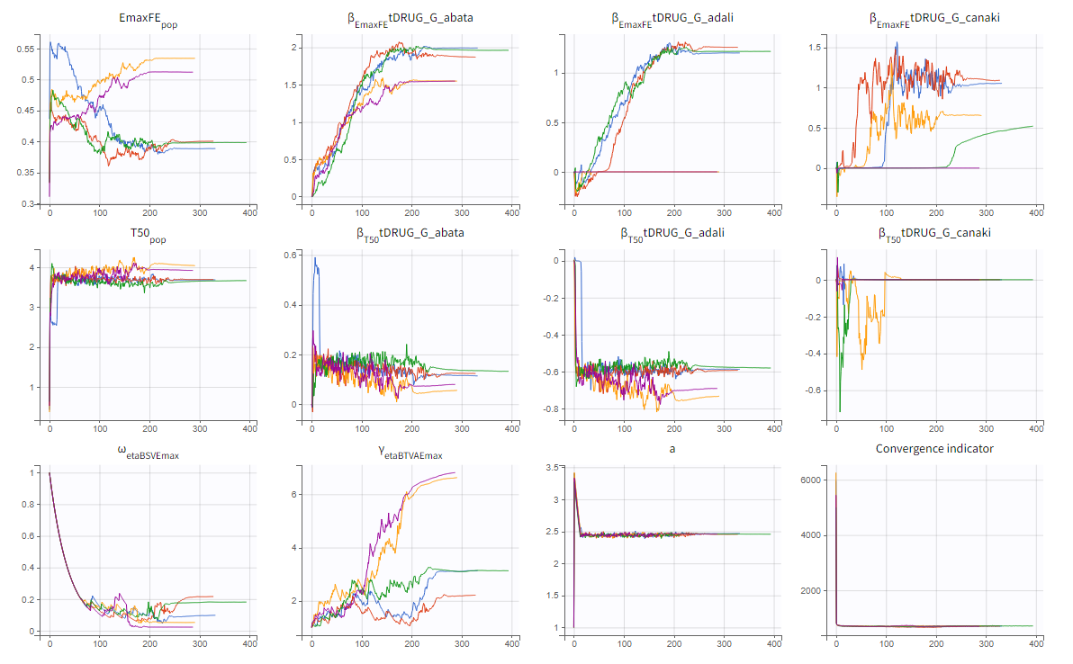
We choose the “variability in the first stage” method and launch the convergence assessment again. This time the convergence is satisfactory.

Results

We can either directly look as the estimated values in the *_rep folders that have been generated during the convergence assessment, or redo the parameter estimation and the estimation of the Fisher information matrix (via linearization for instance) to get the standard errors.

The estimated values are the following:

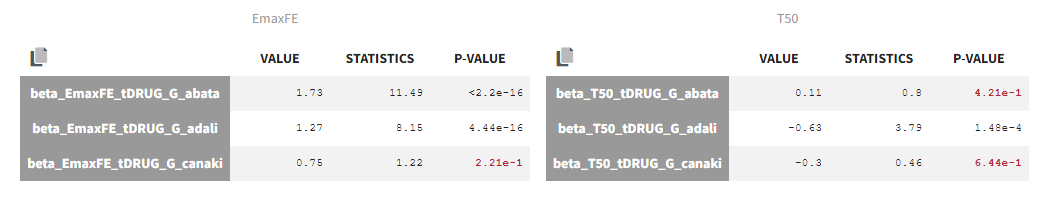
The p-values indicate if the estimated beta parameters, representing the difference between placebo and the other categories, is significantly different from zero. As indicated by the p-value (calculated via a Wald test), the Emax values for Abata and Adali are significantly different from the Emax for placebo. On the opposite, given the data, the Emax value for Canaki is not significantly different from placebo. Note that when analyzing the richer individual data for Canaki, the efficacy of Canaki had been found significantly better than that of placebo (Alten, R. et al. (2011). Efficacy and safety of the human anti-IL-1β monoclonal antibody canakinumab in rheumatoid arthritis: results of a 12-week, Phase II, dose-finding study. BMC Musculoskeletal Disorders, 12(1), 153.). The T50 values are similar for all compounds except Adali.

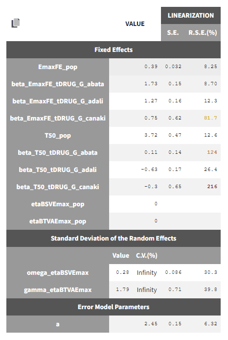
The between study variability of Emax is around 28%. The between treatment arm variability is gamma_etaBTAVEmax = 1.79. In the model, the BTAV gets divided by the square root of the number of individuals per arm. If we consider a typical number of individual per arm of 200, the between treatment arm variability is around 12%.

Note that after setting the random effects of BSVEmax_pop and BTAVEmax_pop equal to 0 we obtain for omega_etaBSVEmax and gamma_etaBTAVEmax Infinity in the C.V.(%). The coefficient of variation is defined as the quotient of the standard deviation and the mean. We therefore divide by 0.

Model diagnosis

We next estimate the study parameters (i.e individual parameters via mode task) and generate the graphics: no model mis-specification can be detected in the individual fits, observations versus predictions, residuals, and other graphics:

Individual fits

Observation versus prediction

Note that all graphics use the transformed observations and transformed predictions.

Alternate models

One could try a more complex model including BSV and BTAV on T50 also. We leave this investigation as hands-on for the reader. The results are the following: the difference in AIC and BIC between the 2 models is small and some standard errors of the more complex model are unidentifiable. We thus decide to keep the simpler model.

Covariate search

The between study variability originates from the different inclusion criteria from study to study. To try to explain part of this variability, we can test adding the studied population characteristics as covariates. The available population characteristics are the mean number of swollen joints, the mean C-reactive protein level and the mean disease duration.
As these covariates differ between arms, they appear in the IOV window. To center the distribution of covariates around a typical value we first transform the covariates using a reference value:

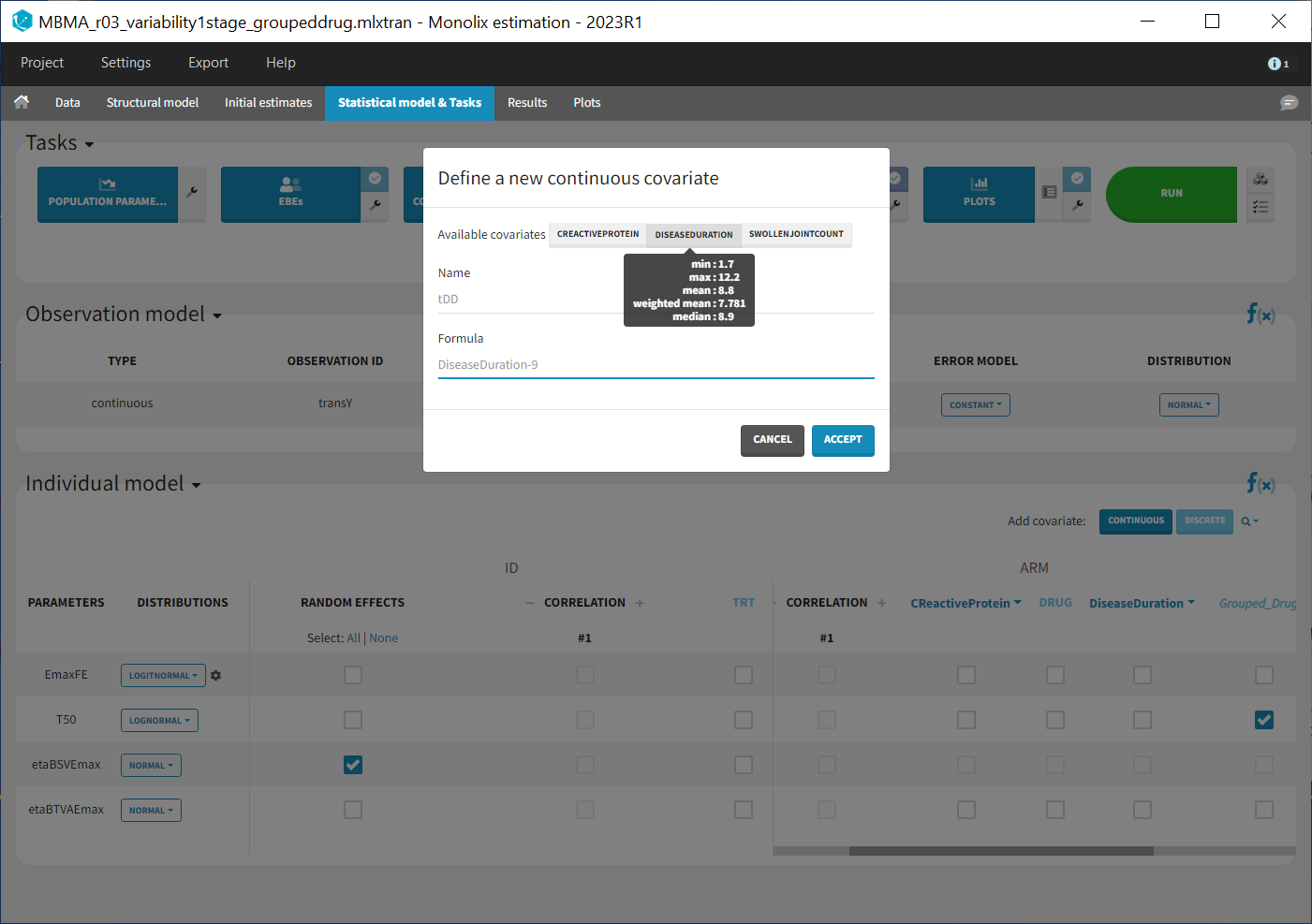
We then include them one by one in the model on the Emax parameter. We can either assess their significance using a Wald test (p-value in the result file, calculated with the Fisher Information Matrix Task), or a likelihood ratio. The advantage of the Wald test is that it requires only one model to be estimated (the one with the covariate) while the likelihood ratio requires both models (with and without covariate) to be estimated. The p-values of the Wald test testing if the beta’s are zero are:

Disease duration: p-value=0.68 (not significant)
C-reactive protein level: p-value=0.39 (not significant)
Swollen joint count: p-value=1.1 (not significant)

The likelihood ratio test also indicates that none of these covariates is significant. We thus do not include these covariates in the model.

Final model overview

The final model has an Emax structural model, with between study and between treatment arm variability on Emax, and no variability on T50. No covariates are included. One Emax and one T50 population parameter per type of treatment (placebo, abata, adali and canaki) is estimated (via the beta parameters). The final run is available in the material (see top of the page) and is called MBMA_r02_variability1stage.mlxtran.

Simulations for decision support

Comparison of canaki efficacy with drugs on the market

We now would like to use the developed model to compare the efficacy of Canaki with the efficacy of Abata and Adali. Has Canaki a chance to be more effective? To answer this question, we will perform simulations using the simulation application Simulx.

To compare the true efficacy (over an infinitely large population) of Canaki with Abata and Adali, we could simply compare the Emax values. However the Emax estimates are marred with uncertainty, and this uncertainty should be taken into account. We will thus perform a large number of simulations for the 3 treatments, drawing the Emax population value from its uncertainty distribution. The BSV, BTAV and residual error will be ignored (i.e set to 0) because we now consider an infinitely large population, to focus on the “true efficacy”.

Before being able to run simulations, we need to export the final project from Monolix to Simulx

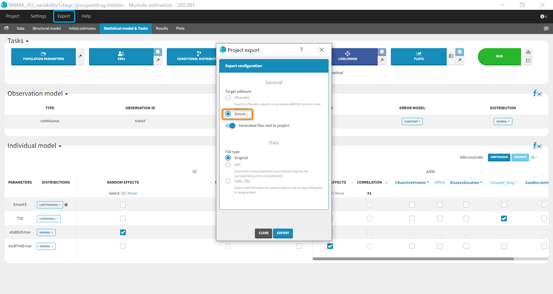
All the information contained in the Monolix project will be transferred to Simulx. This includes the model (longitudinal and statistical part), the estimated population parameter values and their uncertainty distribution and the original design of the dataset used in Monolix (number of individuals, treatments, observation times). Elements containing these information are generated automatically in the “Definition” tab of the created Simulx project. It is possible to reuse these elements to setup a simulation in the “Simulation” tab or create new elements to define a new simulation scenario.

Among the elements created automatically, there is the occasion structure imported from the Monolix dataset. The first step is to delete this occasion element, as we don’t need it for simulations. Go to the tab Definition > Occasions and click on the “delete” button.

To compare the efficacy of Canaki versus Abata and Adali, we will simulate the ACR20 over 52 weeks in 4 different situations (i.e simulation groups) corresponding to Canaki, Abata, Adali and also placebo.

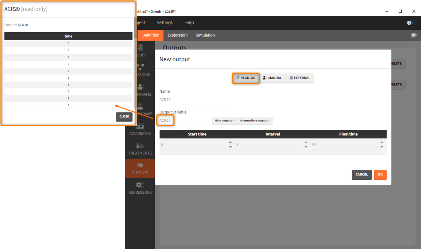
Let’s first define the output. In Monolix we were working with the transformed prediction of ACR20 because of the constraints on the error model. As here we neglect the error model and concentrate on the model prediction, we can directly output the (untransformed) ACR20, at each week.

The definition of the output variable against which we will assess the efficacy of the treatments looks as follows. We output ARC20 on a regular grid from time 0 to week 52

We then need to define the applied treatments, that appear in the model as a categorical covariate. This can be done directly in the covariates tab. We need to define 4 different elements, each corresponding to one of the 4 treatments we want to simulate.

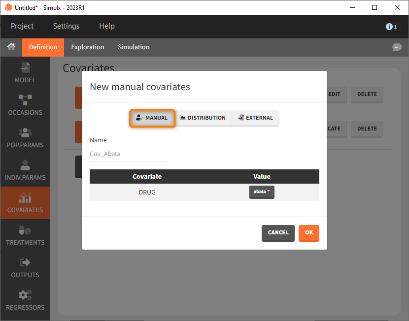
The definition of the other treatments that are not shown in the screenshot above is made analogously.

Last, we define a regressor representing the number of subjects per study. We will see later that this information needs to be defined but will actually not influence the simulations.

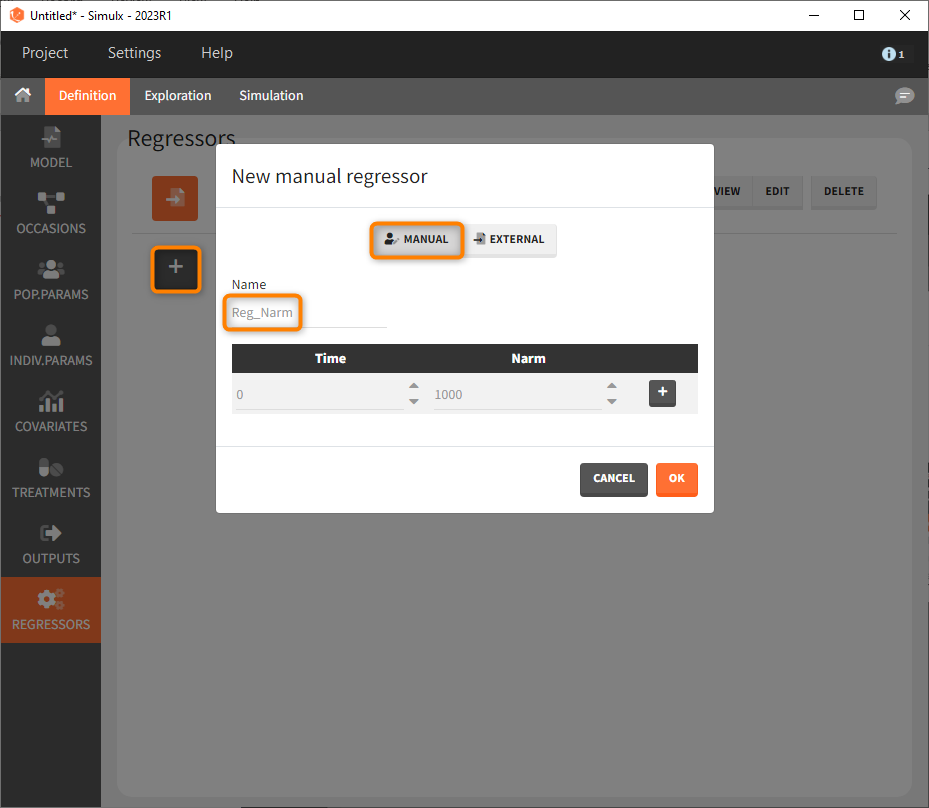
As a first step, we simulate the ACR20 of each treatment using the estimated Emax and T50 values and neglecting the uncertainty. We thus define 4 individuals (i.e studies), one with each treatment:

After defining the output, regressor and treatment variables, we move to the simulation tab.

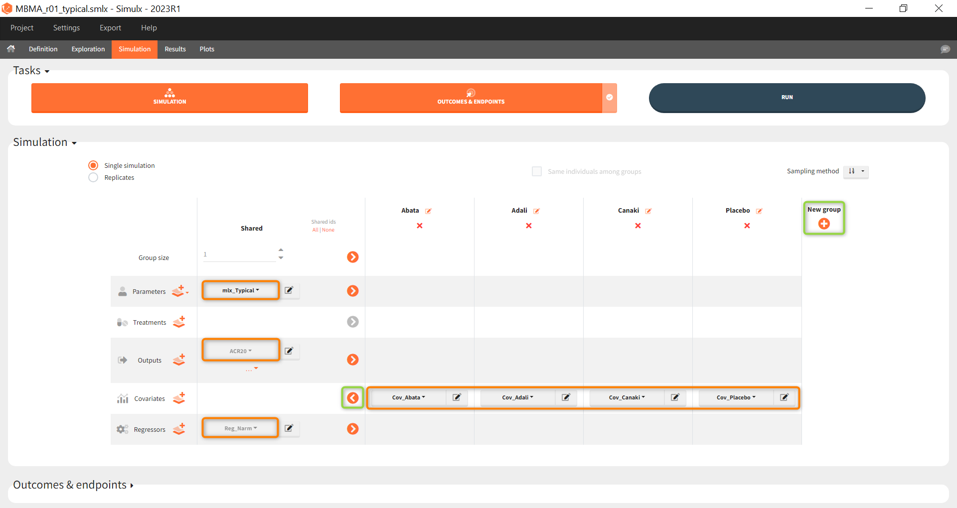
As a first step, we simulate the ACR20 of each treatment using the estimated Emax and T50 values and neglecting the uncertainty. We thus define simulations(i.e studies), one for each treatment.

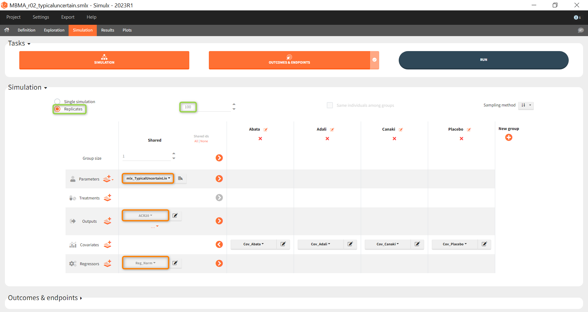
We set 1 as the group size since we want to simulate only one study per treatment. As parameter we select mlx_typical (version 2023 only). This element contains the populations parameters of the last Monolix run, where the standard deviations of the random effects are set equal 0. This allows to simulate a typical study, ignoring the BSV and BTAV. As output variable we set the above defined (untransformed) ACR20 vector. By clicking on the plus under “New group”, the previously defined covariates can be set as treatment in the four simulation groups. As regressor we set the element Reg_Narm defined previously. In theory, the number of subjects in the treatment arms determines the variability between the treatment arms. When the number of subjects goes to infinity, meaning Narm → ∞, the variability converges to 0, meaning etaBTAV/(sqrt(Narm) → 0 . Since we want to describe an ideal scenario, we can set the number of subjects very high. However, we have chosen the element mlx_typical as parameter for the simulation, which already sets the random effects (etaBSV and etaBTAV) and their standard deviation equal to 0. Thus, in practice, Reg_Narm has no effect on the simulation.

After running the simulation, we find in the “Output distribution” tab of the Plot section the response curves of the 4 treatment groups shown in four subplots. To overlay the curves into a single plot, the “merged splits” can be activated in the “Stratify” panel. In addition, by applying the legend toggle in the plot settings and optionally modifying the colors of the treatment arms in the stratification tab, we obtain the following plot:

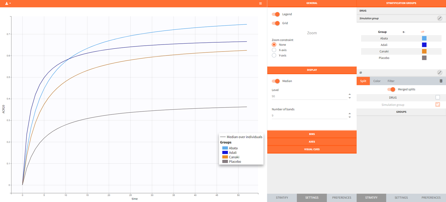
The simulation gives in the generated plot already a first impression of the efficacy of Canaki (orange curve) compared to the other treatments.

By defining outcomes and endpoints, this impression can be quantified.

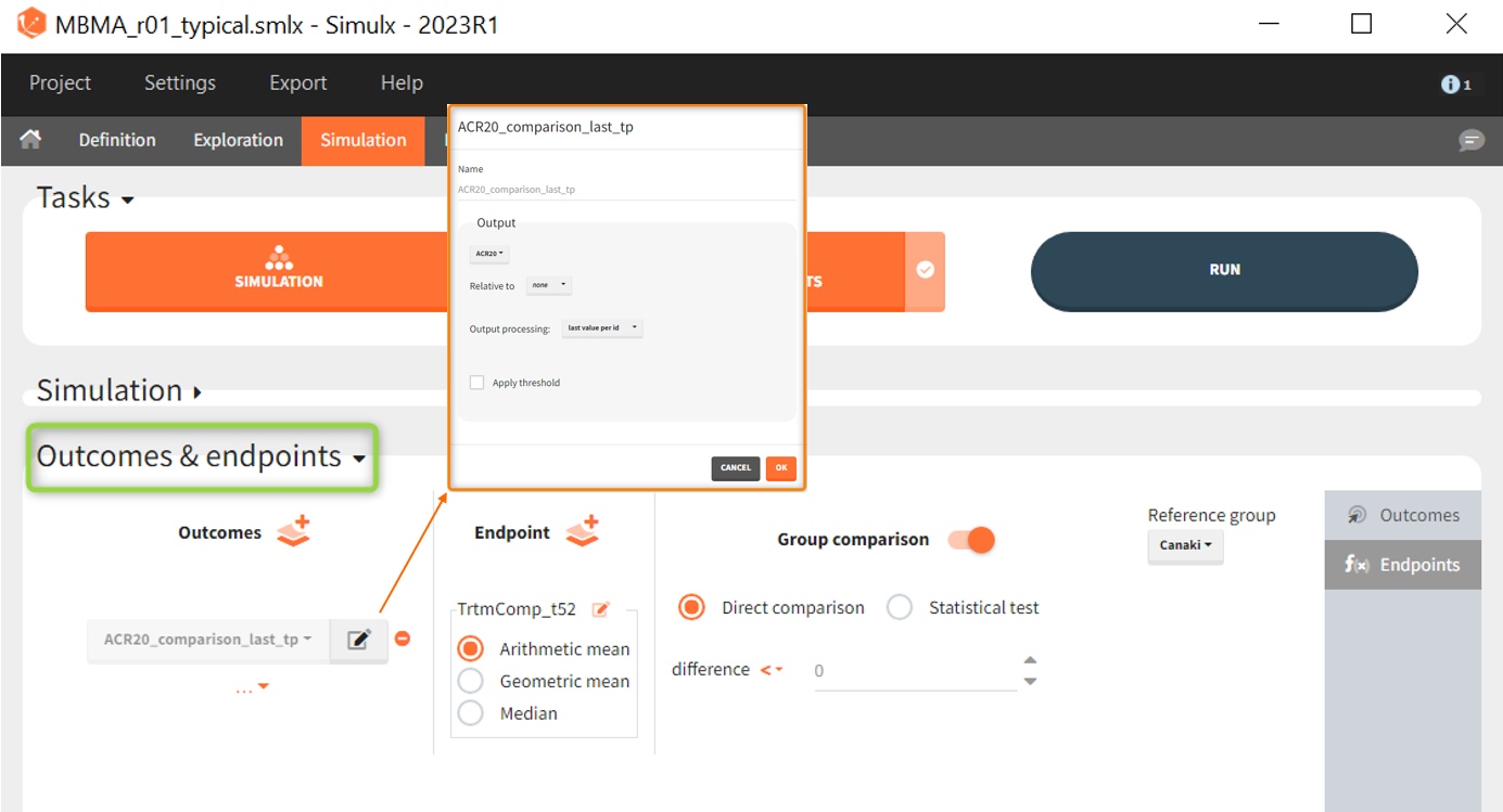
As outcome we define ACR20 at the last time point t = 52. The endpoint can be the arithmetic, geometric mean or median within each simulation group. As we simulate only one study per group, this choice does not matter and the endpoint will be equal to the outcome. We then choose to compare the groups comparing directly the ARC20 values and using Canaki as the reference group. Since the efficacy of Canaki shall be compared with treatments on the market, we set the relation < 0. If the result is negative, Canaki is considered more effective, at =0 it is considered equivalent (at the last time point) and > 0 it is considered insufficient. Written as a formula, we expect the following realtion as a successful experiment outcome:

$$\textrm{Adali_ACR20_t52 } – \textrm{Canaki_ACR20_t52 } \le 0 \Longleftrightarrow \textrm{Canaki_ACR20_t52 } \ge \textrm{Adali_ACR20_t52} $$

The formula is analogous for the treatments Abata compared to Canaki.

In the simulation tab of the results section are summary tables of the simulations per treatment arm, as well as a list of the individual parameters. The endpoint tab of the results includes the arithmetic mean of ACR20 at the last time point t=52. The “StandardDeviation” column, or row, of the Endpoints[Table] tab, or Endpoints[Summary] tab, shows NaN since we have set the samplesize n, which corresponds to the number of studies, equal 1. In the group comparison tab you can find the table with the calculated mean difference of the treatment arms vs. the reference Canaki. The “Success” column indicates whether the comparison can be interpreted as successful. If the difference is < 0, a green check mark appears in the column, if not, a black cross appears.

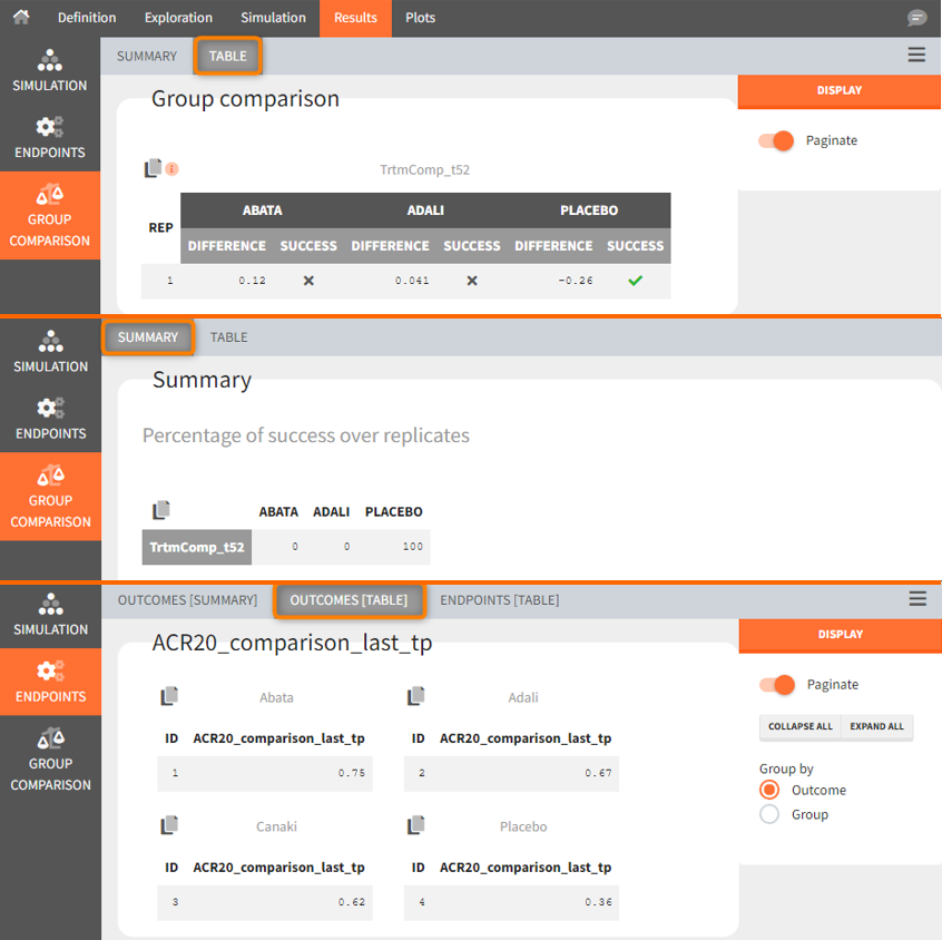
We see that the mean difference between Abata and Canaki, or Adali and Canaki, respectively, is positive. This means that for the 2 treatment groups, ACR20 for Abata or Adali was higher than Canaki at week 52. This suggests that in the ideal case we simulated (infinitely large population), Canaki is less effective than these 2 treatments already on the market. In the Placebo vs. Canaki comparison, however, we see a negative difference, which is also consistent with the above plot of the effect curve. Canaki has at week 52 a higher ACR20 value than Placebo,. Therefore, it can be concluded that Canaki performs better than Placebo, which was expected.

Next, we would like to calculate a prediction interval for the true effect, taking into account the uncertainty of the population parameters estimated by Monolix. To do so, we save the Simulx project under a new name, and make the following changes to the settings:

create 100 replicates of the scenario and
change the population parameter from mlx_Typical to mlx_TypicalUncertain (version 2023 only). This element contains the estimated variance-covariance matrix of the populations parameters of the final Monolix run with standard deviations of the random effects equal to 0. It enables to simulate a typical subject (meaning a study) with different population parameter values for each replicate, such that the uncertainty of population parameters is propagated to the predictions.

The defined outcomes and endpoints remain the same. The objective is to see what happens to the conclusion of the success criterion when we repeat the scenario 100 times with different sets of population parameters.

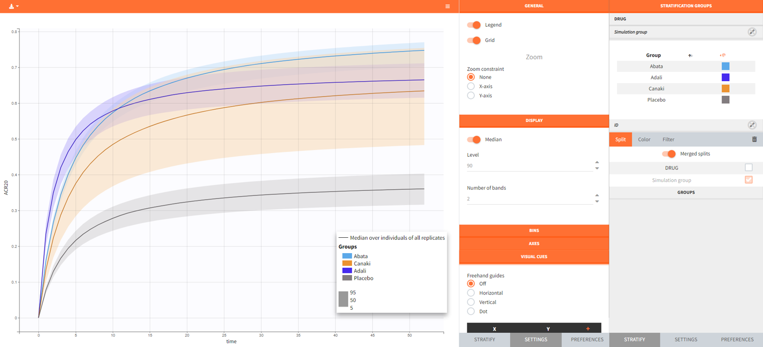
The output distribution plot again shows the response curve, but now with the percentiles of the simulated data for all calculated replicates. The “number of bands” in Display can be set to 2 and the subplots merged to easy the comparison.

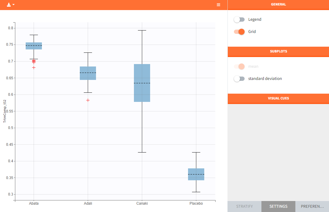
In the “Endpoint distribution” tab of the generated plots, we see the distribution over all replicates of ACR20 at week 52 of all 4 treatment groups. It is clearly visible that the treatments with the active compounds are more effective than the placebo group. However, the mean value of Canaki after 100 replicates is below the mean values of Abata and Adali.

Note: The thickness of the bands in the “Output distribution” plot as well as the length of the box + whiskers of the boxplot of the “Endpoint distribution” plot of Canaki can be explained by the fact that there was much less data available compared to the other treatments. This leads to a larger uncertainty of the true effect of Canaki in comparison to the other drugs.

If we go back to the results section, we find analogous tables as in the simulation performed before, but this time with results per replicate.

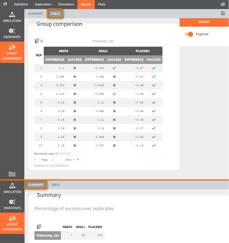
Using the summary table we can conclude that at time point t= week 52, given the estimated populations parameter:

out of 100 repetitions the relation Canaki_ACR20_t52 > Abata_ACR20_t52 was met only 7 times ⟹ we have a 7% chance that Canaki performs better than Abata
out of 100 repetitions the relation Canaki_ACR20_t52 > Adali_ACR20_t52 was met only 36 times ⟹ we have a 36% chance that Canaki performs better than Adali
out of 100 repetitions the relation Canaki_ACR20_t52 > Placebo_ACR20_t52 was met 100 times ⟹ we have a 100% chance that Canaki performs better than Placebo

This finding supported the decision not to continue with clinical development of canakinumab in RA, according to:

Demin, I., Hamrén, B., Luttringer, O., Pillai, G., & Jung, T. (2012). Longitudinal model-based meta-analysis in rheumatoid arthritis: an application toward model-based drug development. Clinical Pharmacology and Therapeutics, 92(3), 352–9.

Conclusion

Model-informed drug development

Model based meta-analysis supports critical decisions during the drug development process. In the present case, the model has shown that chances are low that Canaki performs better than two drugs already on the market. As a consequence the development of this drug has been stopped, thus saving the high costs of the phase III clinical trials.

MBMA with Monolix and Simulx

This case study also aims at showing how Monolix and Simulx can be used to perform longitudinal model-based meta-analysis. Contrary to the usual parameter definition in Monolix, the weighting of the between treatment arm variability imposes to split the parameters into their fixed term and their BSV and BTAV terms, and reform the parameter in the model file. Once the logic of this model formulation is understood, the model set up becomes straightforward. The efficient SAEM algorithm for parameter estimation as well as the built in graphics then allow to efficiently analyze, diagnose and improve the model.
The inter-operability between Monolix and Simulx permits to carry the Monolix project over to Simulx to easily define and run simulations.

Natural extensions

In this case study, continuous data were used. Yet, the same procedure can be applied to other types of data such as count, categorical or time-to-event data.

Guidelines to implement your own MBMA model

Setting up your data set

Your data set should usually contain the following columns:

STUDY: index of the study/publication. It is equivalent to the ID column for individual-level data.
ARM: index of the arm (preferably continuous integers starting at 0). There can be an arbitrary number of arms (for instance several treated arms with different doses) and the order doesn’t matter. This column will be used as equivalent to the occasion OCC column.
TIME: time of the observations
Y: observations at the study level (percentage, mean response, etc)
transY: transformed observations, for which the residual error model is constant
Narm: number of individuals in the arm. Narm can vary over time
Covariates: continuous or categorical covariates that are characteristics of the study or of the arm. Covariates must be constant over arms (appear in IOV window) or over studies (appear in main window).

Frequent questions about the data set

Can dropouts (i.e. a time-varying number of individuals per arm) be taken into account? Yes. This can be accounted for without difficulty as the number of subjects per arm (Narm) is passed as a regressor to the model file, a type that allow by definition variations over time.
Can there be several treated (or placebo) arms per study? Yes. The different arms of a study are distinguished by a ARM index. For a given study, one can have observations for ARM=0, then observations for ARM=1, then observations for ARM=2. The index number has no special meaning (for instance ARM=0 can be the treated arm for study 1, and ARM=0 the placebo arm for study 2).
Why should I transform the observations? The observations must be transformed such that an error model from the list (constant, proportional, combined, exponential, etc) can be used. In the example above, we have done two transformations: first we have used a logit transformation, such that the prediction of the fraction of individuals reaching ACR20 will remain in the 0-1 interval, even if by chance a large residual error term is drawn. If we instead consider a mean concentration of glucose for instance, we could use a log-transformation to ensure positive values. Second, we need to multiply each value by the square root of the number of individuals per arm. With this transformation, the standard deviation of the error term is the same for all studies and arms, and does not depend on the number of individuals per arm anymore.

Setting up your model

The set up of your project can be done in four steps

Split the parameters in several terms
Make the appropriate transformation for the parameters
Set the parameter definition in the Monolix interface
Add the transformation of the prediction

Frequently asked questions on setting up the model

Why should I split a parameter in several terms? Because the standard deviation of the BTAV term must usually by weighted by the square root of the number of individuals per arm, this term must be handled as a separate parameter and added to the fixed effect within the model file. Moreover, the fixed effect and its BSV random effect might be split depending on the covariate definition.
How do I know in how many terms should I split my parameter?
- If all covariates of interest are constant over studies: 2. In this case, the parameters can be split into a (fixed effect + BSV) term and a (BTAV) term. The model file would for instance be (for a logit distributed parameter):

[LONGITUDINAL]

input = {paramFE_BSV, etaBTAVparam, Narm}

Narm = {use=regressor}

EQUATION:

tparam = logit(paramFE_BSV)

tparamRE = tparam + etaBTAVparam/sqrt(Narm)

paramRE = 1 / (1+ exp(-tparamRE))

=> Impact on the interface: In the GUI, paramFE_BSV would have both a fixed effect and a BSV random effect. Covariates can be added on this parameter in the main window. The etaBTAVparam fixed effect should be enforced to zero, the BSV disabled and the BTAV in the IOV part enabled.

- If one covariate of interest is not constant over studies: 3. This was the case for our case study (the DRUG covariates was constant over arms, not studies). Here, the parameters must be split into a fixed effect term, a BSV term and a BTAV term. The model file would for instance be (for a logit distributed parameter):

[LONGITUDINAL]

input = {paramFE, etaBSVparam, etaBTAVparam, Narm}

Narm = {use=regressor}

EQUATION:

tparam = logit(paramFE)

tparamRE = tparam + etaBSVparam + etaBTAVparam/sqrt(Narm)

paramRE = 1 / (1+ exp(-tparamRE))

=> Impact on the interface In the GUI, paramFE has only a fixed effect (BSV random effect must be disabled in the variance-covariance matrix). Covariates can be added on this parameter in the IOV window. The fixed effect value of etaBSVparam must be enforced to zero. The etaBTAVparam fixed effect should be enforced to zero too, the BSV disabled and the BTAV in the IOV part enabled.

Why shouldn’t I add covariates on the etaBTAVparam in the IOV window? Covariates can be added on etaBTAVparam in the IOV window. Yet, because the value of etaBTAVparam will be divided by the square root of the number of individuals in the model file, the covariate values in the data set must be transformed to counter-compensate. This may not always be feasible:
- If the covariate is categorical (as the DRUG on our example), it is not possible to compensate and thus the user should not add the covariate on the etaBTAVparam in the GUI. A splitting in 3 terms is needed.
- If the covariate is continuous (weight for example), it is possible to counter-compensate. Thus, if you add the covariates on the etaBTAVparam in the GUI, the covariate column in the data set must be multiplied by $\sqrt{N_{ik}}$ beforehand. This is a drawback, however this modeling has less parameters without variability and may thus converge more easily.

How should I transform the parameter depending on its distribution? Depending on the original parameter distribution, the parameter must first be transformed as in the following cases:

For a parameter with a normal distribution, called paramN for example, we would have done the following:

; no transformation on paramN as it is normally distributed
tparamN = paramN
; adding the random effects (RE) due to between-study and between arm variability, on the transformed parameter
tparamNRE = tparamN + etaBSVparamN + etaBTAVparamN/sqrt(Narm)
; no back transformation as tparamNRE already has a normal distribution
paramNRE = tparamNRE

Note that the two equalities are not necessary but there for clarity of the code.

For a parameter with a log-normal distribution, called paramLog for example (or T50 in the test case), we would have done the following:

; transformation from paramLog (log-normally distributed) to tparamLog (normally distributed)
tparamLog  = log(paramLog) 
; adding the random effects (RE) due to between-study and between arm variability, on the transformed parameter 
tparamLogRE = tparamLog  + etaBSVparamLog + etaBTAVparamLog/sqrt(Narm)
; transformation back to have paramLogRE with a log-normal distribution
paramLogRE = exp(tparamLogRE)

For a parameter with a logit-normal distribution in ]0,1[, called paramLogit for example (or Emax in the test case), we would have done the following:

; transformation from paramLogit (logit-normally distributed) to tparamLogit (normally distributed)
tparamLogit  = logit(paramLogit) 
; adding the random effects (RE) due to between-study and between arm variability, on the transformed parameter 
tparamLogitRE = tparamLogit  + etaBSVparamLogit + etaBTAVparamLogit/sqrt(Narm)
; transformation back to have paramLogitRE with a logit-normal distribution
paramLogitRE = 1 / (1+ exp(-tparamLogitRE))

For a parameter with a generalized logit-normal distribution in ]a,b[, called paramLogit for example, we would have done the following:

; transformation from paramLogit (logit-normally distributed in ]a,b[) to tparamLogit (normally distributed)
tparamLogit  = log((paramLogit-a)/(b-paramLogit))

; adding the random effects (RE) due to between-study and between arm variability, on the transformed parameter 
tparamLogitRE = tparamLogit + etaBSVparamLogit + etaBTAVparamLogit/sqrt(Narm) 
; transformation back to have paramLogitRE with a logit-normal distribution in ]a,b[
paramLogitRE =(b * exp(tparamLogitRE) + a)/ (1+ exp(tparamLogitRE))

How do I set up the GUI? Depending which option has been chosen, the fixed effects and/or the BSV random effects and/or the BTAV random effects of the model parameters (representing one or several terms of the full parameter) must be enforced to 0. Random effects can be disabled by clicking on the RANDOM EFFECTS column and fixed effects by choosing “fixed” after a click in the initial estimates.
Why and how do I transform the prediction? The model prediction must be transformed in the same way as the observations of the data set, using the column Narm passed as regressor.

Parameter estimation

The splitting of the parameters into several terms may introduce model parameters without variability. These parameters cannot be estimated using the main SAEM routine, but instead are optimized using alternative routines. Several of them are available in Monolix, under the settings of SAEM. If the method by default leads to poor convergence, we recommend to test the other methods.

Model analysis

All graphics are displayed using the transformed observations and predictions. These are the right quantities to diagnose the model using the “Observation versus prediction” and “Scatter plot of the residuals”, “distribution of the residuals” and graphics. For the individuals fits and VPC, it may also be interesting to look at the non-transformed observations and predictions. These graphics can be redone in R using the simulx function of the mlxR package. The other diagnostic plots (“Individual parameters vs covariates”, “Distribution over the individual parameters”, “Distribution of the random effects”, and “Correlation of the random effects”) are not influenced by the transformation of the data.