Download data set only | Download all Monolix and Simulx project files | Download Simulx R script
This time-to-event case study represents a detailed modeling and simulation workflow using MonolixSuite applications. It is recommended to read before the Introduction to TTE data and library of models in Monolix.
Another case study on time-to-event data is also available: Case study on veteran lung cancer data set
In this case study, we develop a model for the NCCTG survival data set and study the effect of covariates.
- Introduction
- Data set visualization
- Modeling with Monolix
- Simulations with Simulx
- Conclusion
- Downloads
Introduction
The North Central Cancer Treatment Group (NCCTG) data set records the survival of 228 patients with advanced lung cancer, together with assessments of the patients performance status measured either by the physician and by the patients themselves. The goal of the study was to determine whether patients self-assessment could provide prognostic information complementary to the physician’s assessment.
This data set has been originally presented and analyzed in:
In this case study, we will test several parametric models to capture this data set and evaluate the prognostic performance of the recorded covariates.
Data set visualization
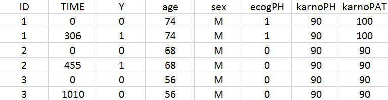
The data set contains 228 patients, including 63 patients that are right censored (patients that left the study before their death). The original data set has been reformatted according to the data set formatting guidelines and includes both the starting time and the time of death or drop out.
To assess the importance of self performance assessment versus physician’s assessment, the following covariates have been recorded:
- ecogPH: ECOG (Eastern Cooperative Oncology Group) performance status assessed by the physician, on a scale from 0 (fully active) to 5 (dead). For information on the scale, click here.
- karnoPH: Karnofsky performance status, assessed by the physician, on a scale from 0 (dead) to 100 (completely healthy). More details about the scale can be found here.
- karnoPAT: Karnofsky performance status, assessed by the patient
- sex: sex of the patient (F for female, M for male)
- age: age of the patient (years)
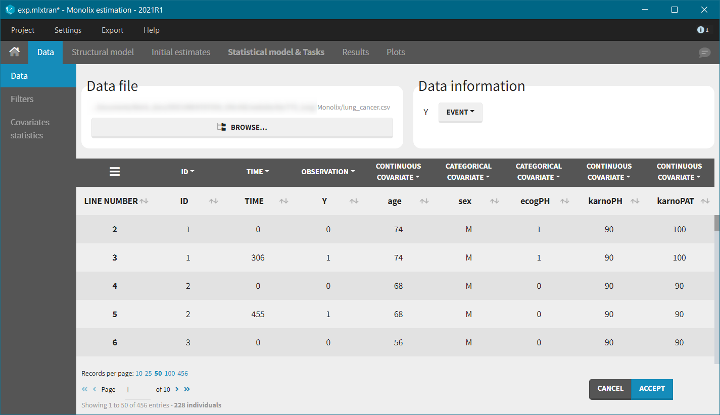
We first use Monolix to visualize the data set. After having opened Monolix, we start a new project and load the data (the covariates must be assigned to continuous covariates or categorical covariates tags). To visualize time-to-event data we must indicate that the data is of the EVENT type in the Data information section.
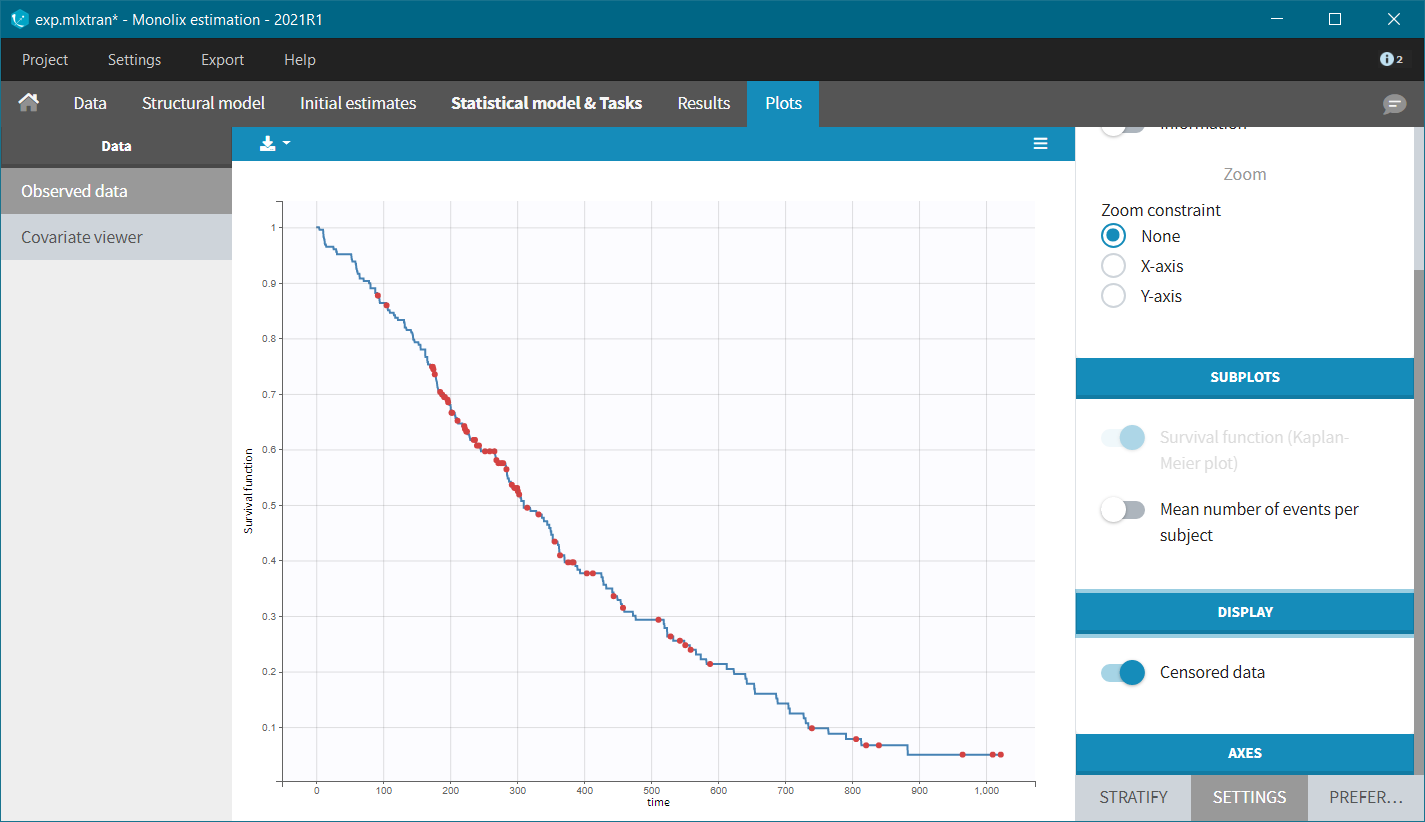
After accepting the dataset, the Kaplan-Meier (KM) estimate of the survival curve is displayed in the Plots tab. In the “Settings” (right panel), we can add the mean number of events curve and display the censored data.
The Kaplan-Meier curve cannot be stratified by “coloring”, but you can split it and then a “merge” with a button that appears. It will merge the plots in one figure with different colors (fixed) for each curve. Add legend to visualize the assignment of colors to each stratification group.
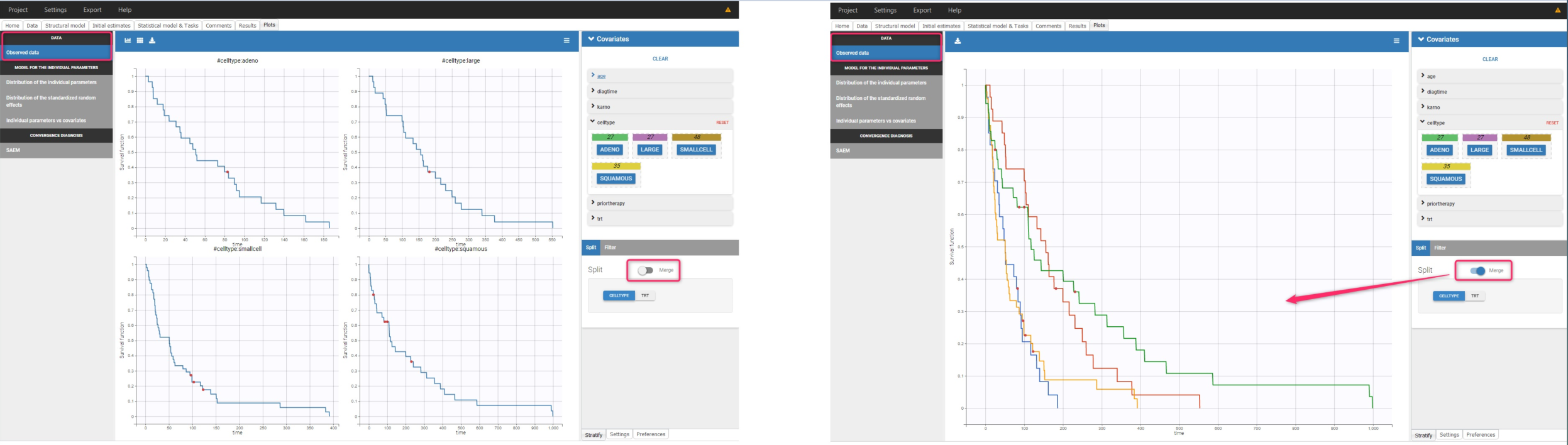
Stratification according to categorical or continuous covariates (groups can be changed) helps to visually check the impact of the covariates. At first sight, it seems that sex, ECOG, karnoPH and karnoPAT influence the survival, while age does not.
sex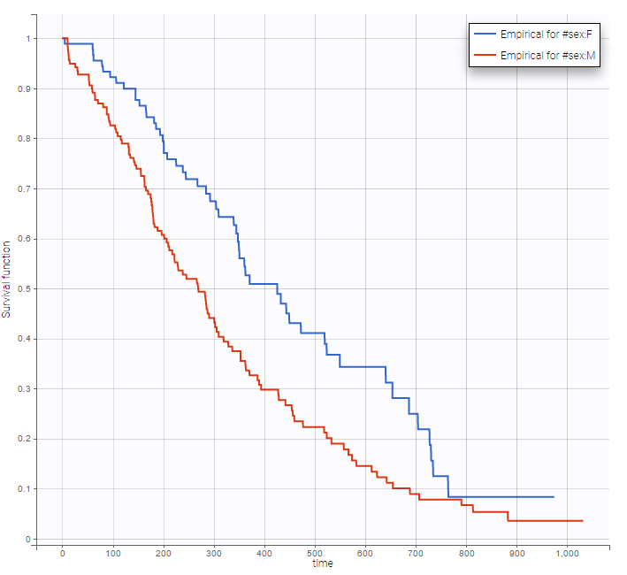 |
Age |
|---|
|
ecogPH |
karnoPH |
karnoPAT |
|---|
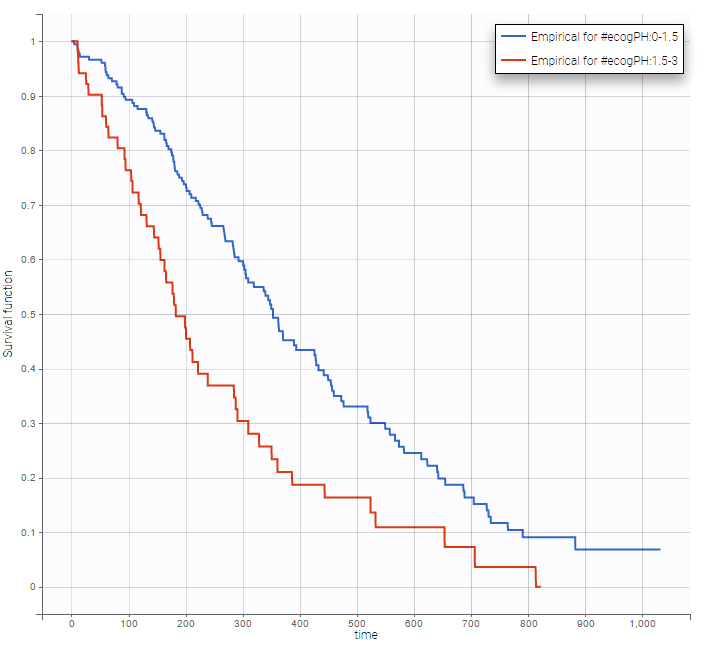
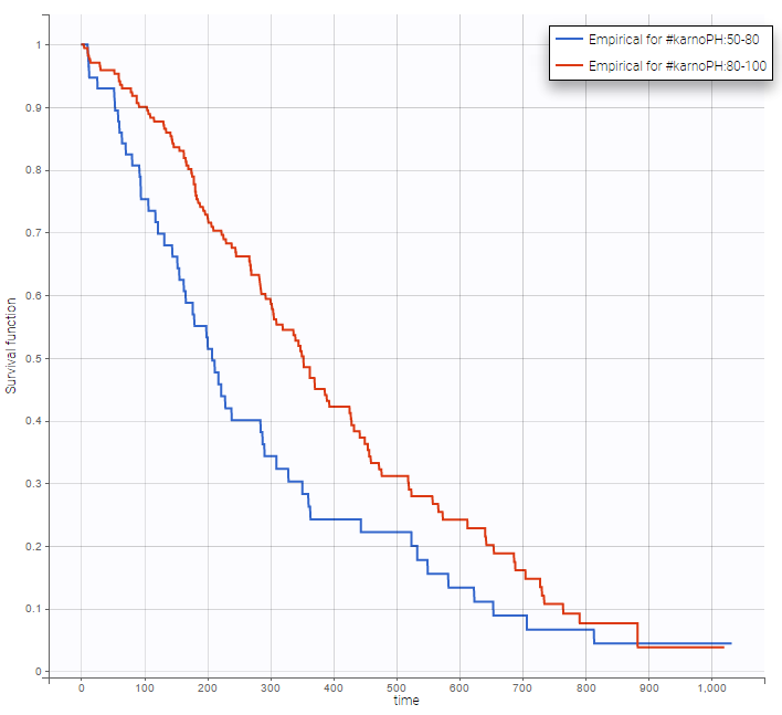
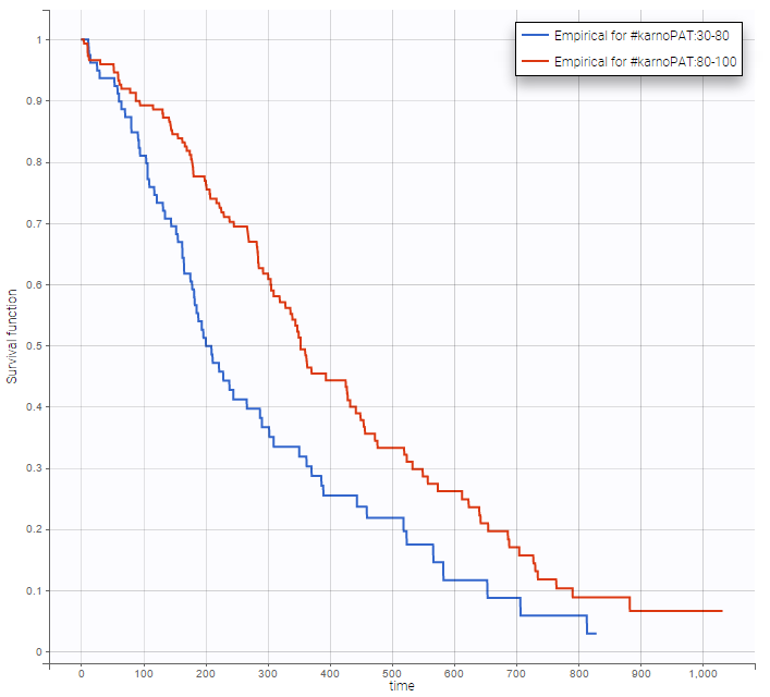
Note that ECOG, karmoPH and karnoPAT are all performance scores and that they are probably strongly correlated.
Modeling with Monolix
Now we develop a model for this data set, and analyse which covariates have the highest prognostic performance. Within the MonolixSuite, only parametric models for time-to-event data are possible (no non-parametric or semi-parametric approaches).
Structural model
We start with the development of the structural model. The typical shape of common parametric survival models has been presented in the Part 1 of the TTE case study, together with the library of common TTE models. From the KM curve visualization, the Weibull, log-logistic, gamma or Gompertz models could be appropriate. We will try each in turn, choosing the files with extensions “_singleEvent.txt” from the library.
For models with 2 parameters, it is common to assume that the shape parameter is the same for all individuals, while the scale parameter can vary from individual to individual. This inter-individual variability can be captured via the effect of covariates and/or via random effects (often called frailty models). Following this strategy, the random effects are disabled for the shape parameters p, s, k and alpha (by clicking on the corresponding diagonal element of the variance-covariance matrix) and kept for the scale parameter Te. We also keep the default log-normal distributions, to ensure positive values of the parameters.
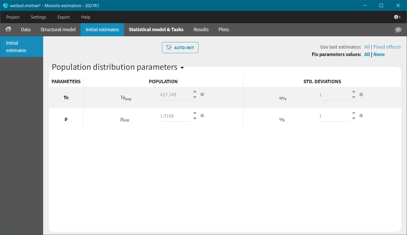
In each model, the scale parameter is the characteristic time Te. Using the KM data visualization, we choose 300 as initial value, i.e the value for which the survival is around 50%. For the shape parameter, we use as initial value 1, according to the typical value chart given on the page of the TTE model library. Starting from the Monolix2021R1 version, the auto-initialization is available also for time-to-event data.
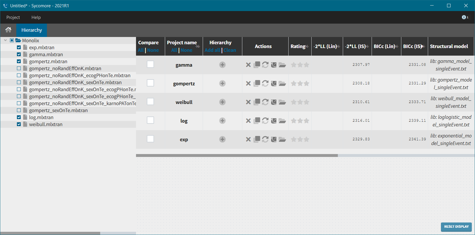
We next launch the estimation tasks for each structural model in turn: estimation of the population parameters, estimation of the individual parameter, estimation of the standard errors via the Fisher Information Matrix, estimation of the log-likelihood and generation of the graphics. The performance of each structural model can then be assessed and compared using the TTE graphic and the log-likelihood values. A Sycomore project helps to organize and compare different models.
After each run, in the Time to Event data graphic, one can calculate the 90% prediction interval for the KM curve given the model (in Settings > Prediction interval) and overlay it on top of the empirical KM curve. It can be interpreted in the same way as a VPC. A summary is presented below:
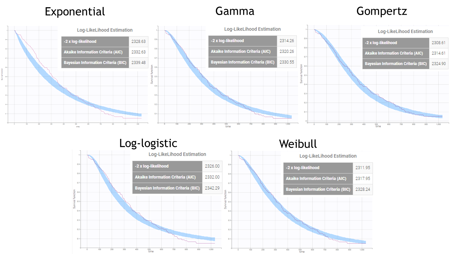
From a visual point of view, the exponential, log-logistic and gamma models can be excluded as they do not capture the shape of the KM curve. The Weibull and Gompertz models are satisfactory, with a slight preference for the Gompertz model, as indicated by the BIC values. We thus choose the Gompertz model as structural model.
Covariate model
We next investigate covariates, added on the Te parameter, can help to explain its inter-individual variability. For didactic purposes, we will perform the covariate search by hand and stepwise.
In Monolix, using a backward covariate search approach is especially powerful. Indeed, after having calculated the s.e, a Wald test is performed to test the significance of each covariate. Thus it is sufficient to estimate the parameters of the model including all covariates relationships to get a p-value for each relationship, without having to estimate the submodels with one covariate relationship less. Following this strategy, we will estimate the model with all available covariates on Te and stepwise remove the less significant relationship, until all remaining covariates are significant. The AIC and BIC will also be monitored in parallel.
We thus add all covariates on the Te parameter in the “Covariate model” section, which corresponds to the following model for Te:
$$T_{e,i}=T_{e,\textrm{pop}}e^{\beta_{\textrm{sex}}[\textrm{if sex=M}] + \beta_{\textrm{age}}\times\textrm{age} + \beta_{\textrm{ecogPH}}\times\textrm{ecogPH} + \beta_{\textrm{karnoPH}}\times\textrm{karnoPH} + \beta_{\textrm{karnoPAT}}\times\textrm{karnoPAT}} e^{\eta_i}$$
The table below summarizes the stepwise covariate removal, based on the p-values, and AIC/BIC: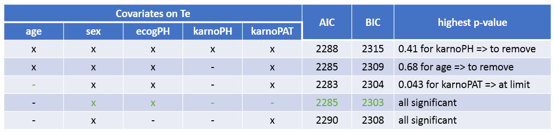
The models with (sex, ecogPH, karnoPAT) and (sex, ecogPH) have similar AIC and BIC values. Yet the model with (sex, ecogPH, karnoPAT) has a high condition number (around 300), we thus prefer the (sex, ecogPH) model.
Final model
Our final model includes a Gompertz structural model, and the covariates sex, and ecogPH on the scale parameter Te. The model improvement when karnoPAT is included in addition to ecogPH is very small indicating that a self-assessment of the performance status by the patient permits only a slightly better prognosis, compared to using the physicians ECOG performance status evaluation only. In the original study including more patients and different types of cancer, the value of patient self-assessment was higher.
The estimated parameters are below. The r.s.e are reasonable.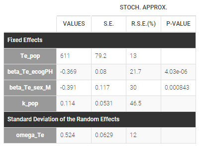
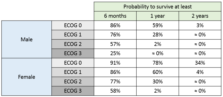
The 90% prediction interval for the KM curve shows that the data is properly captured. The other graphics do not hint at any model mis-specification. 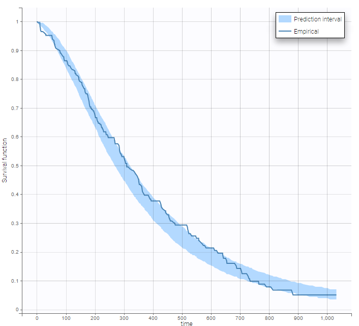 For a given sex and a given ecogPH score, we can easily calculate analytically the typical hazard and the associated Gompertz model survival. From the survival function, we calculate the probability to survive at least 6 months (180 days), 1 year (365 days), or 2 years (730 days) depending on the sex and ECOG score:
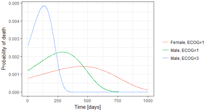
The probability density function of the death event can also be easily calculated analytically as the product of the hazard and the survival functions, for a given sex and ECOG score. Below we show the probability of death with respect to time for three different cases. The plot can also be interpreted as the distribution of death times in each of the three sub-populations.
Simulations using Simulx GUI
The model developed in Monolix can be used to simulate new populations. Here, we would like to simulate three new patients cohorts (with different covariates compared to the original data set). The three cohorts have the following characteristics:
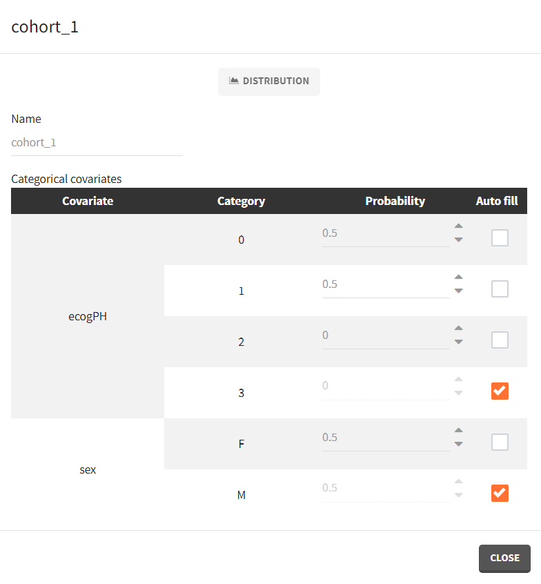
- cohort 1: 50% male / 50% female, good ECOG scores (0 or 1)
- cohort 2: 50% male / 50% female, poorer ECOG scores (2 or 3)
- cohort 3: 90% male / 10% female, good ECOG score (0 and 1)
To simulate these three cohorts, we first import the final Monolix project to Simulx. Model (structural and statistical), parameters (population and individual), outputs and covariates are imported from the Monolix project and its dataset. In the Simulation tab of Simulx, the default scenario corresponds to re-simulating a dataset used in the Monolix project.
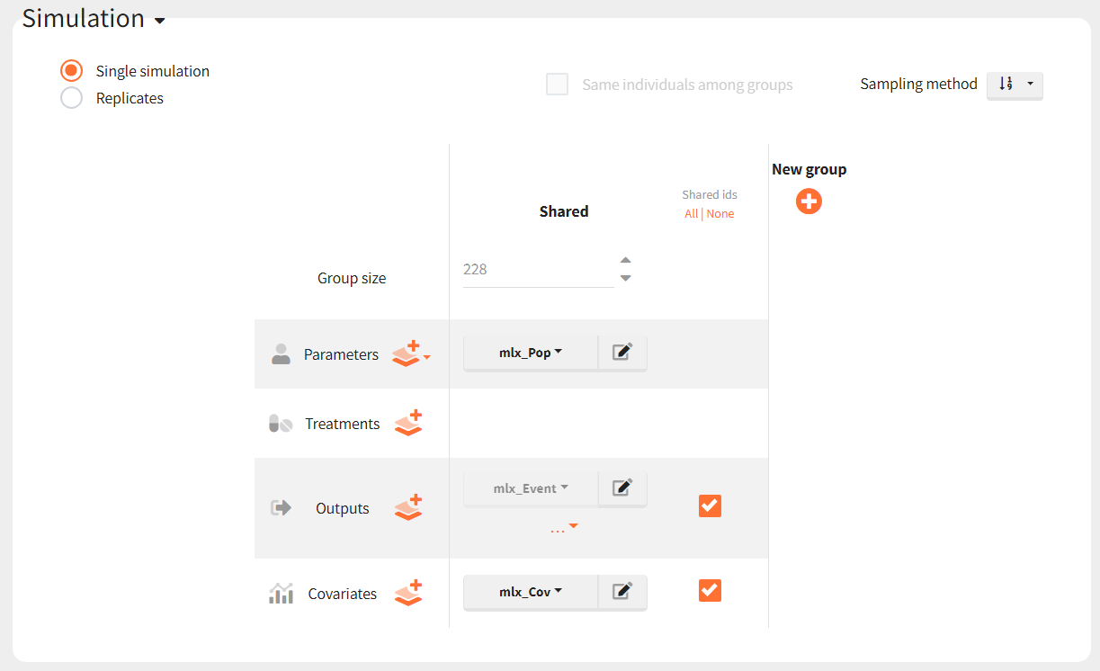
To simulate new cohorts, we create three groups, each with a group specific covariate element corresponding to one of the covariate element specified above. For example, cohort 1 is defined as follows:
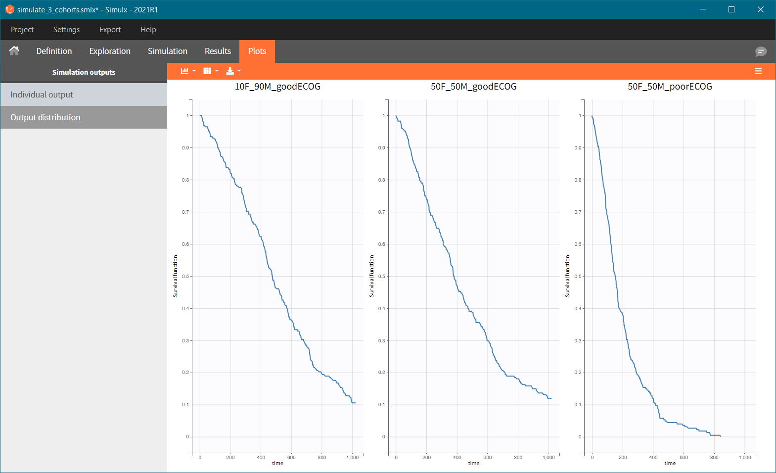
After running the scenario, the three Kaplan-Meier curves (one per group) are displayed in the Plots tab.
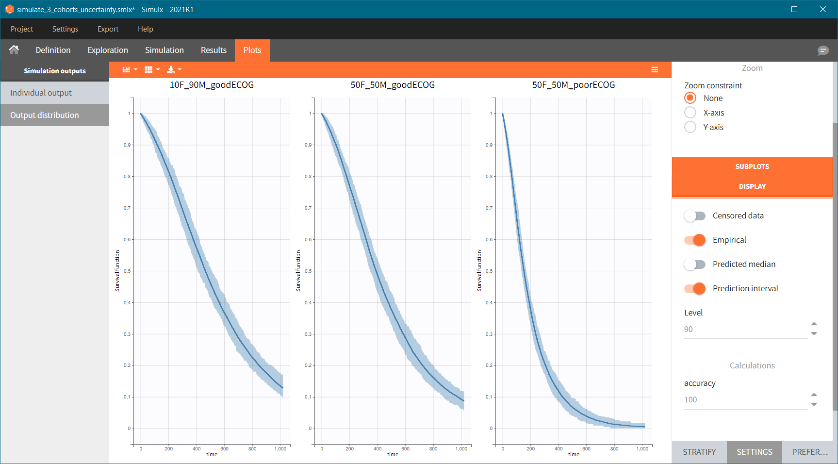
Because the time of death is a random variable, several simulations of the same population will lead to different survival curves. We can assess the uncertainty of the survival curve by doing replicates – change “Single simulation” to “Replicates” in the scenario definition. The outputs represents now the prediction interval for the Kaplan-Meier curve:
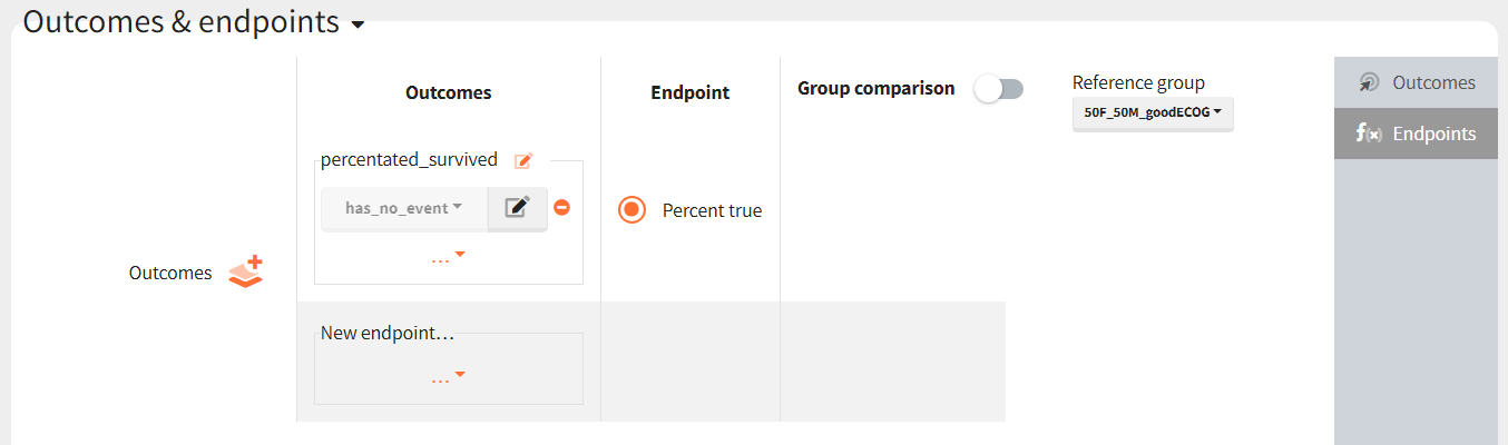
To quantitatively compare the median survival we use the post-processing tool in Simulx: outcomes & endpoints. It allows to calculate how many individuals survive a certain time and asses the uncertainty of this result (when simulating replicates). For example, we can create an outcome to check if an individual “has no event” between the start of the observation (time = 0) and the end (time = 750).
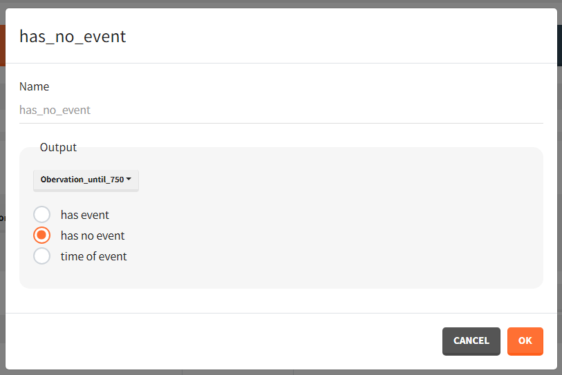
Then, this outcome is used in the definition of an endpoint: percent true
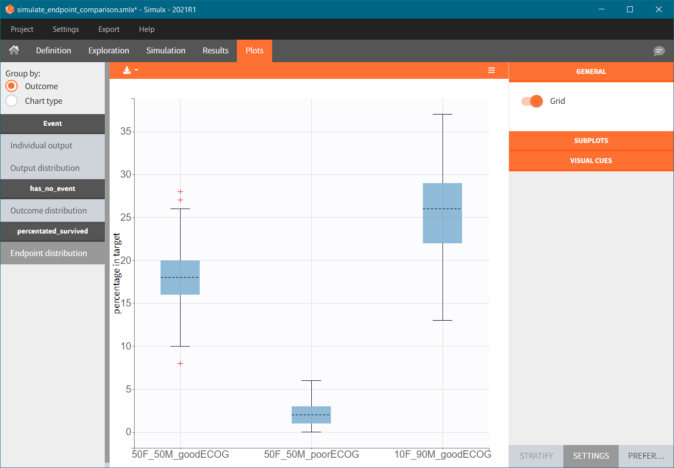
The results are presented in the results tables and as a boxplot in the plots tab:
Simulations via scripting with RsSimulx
The documentation on the RsSimulx R-function can be found here: https://simulx.lixoft.com/rssimulx/
Simulation of three new patients cohorts (with different covariates compared to the original data set):
- cohort 1: 50% male / 50% female, good ECOG scores (0 or 1)
- cohort 2: 50% male / 50% female, poorer ECOG scores (2 or 3)
- cohort 3: 90% male / 10% female, good ECOG score (0 and 1)
To simulate these three cohorts, we create three groups, each defined via a data frame of the individuals covariates, and pass them as simulx() input argument. The simulation is done via the simulx() function which returns a R object containing the result of the simulation (time of death for each individual). We can then pass this object to kmplotmlx to obtain the Kaplan-Meier survival curves.
For cohort 1, the R code reads:
# defining the path to the mlxtran project file
project.file <- "./monolix_project/43_gompertz_all_nokarnoPH_noage_nokarnoPAT.mlxtran"

#========== defining group 1
# covariate data frame for group 1, with column id and one column per covariate
cov1 <- data.frame(id=1:228,
 sex = c(rep("F",114),rep("M",114)),
 ecogPH = rbinom(n=228, size=1, prob=0.5),
 )

#============= calling simulx for group 1
res1 <- simulx(project = project.file,
               parameter = cov1)
We then combine the output objects into one and plot with:
#============= plotting the KM survival curve
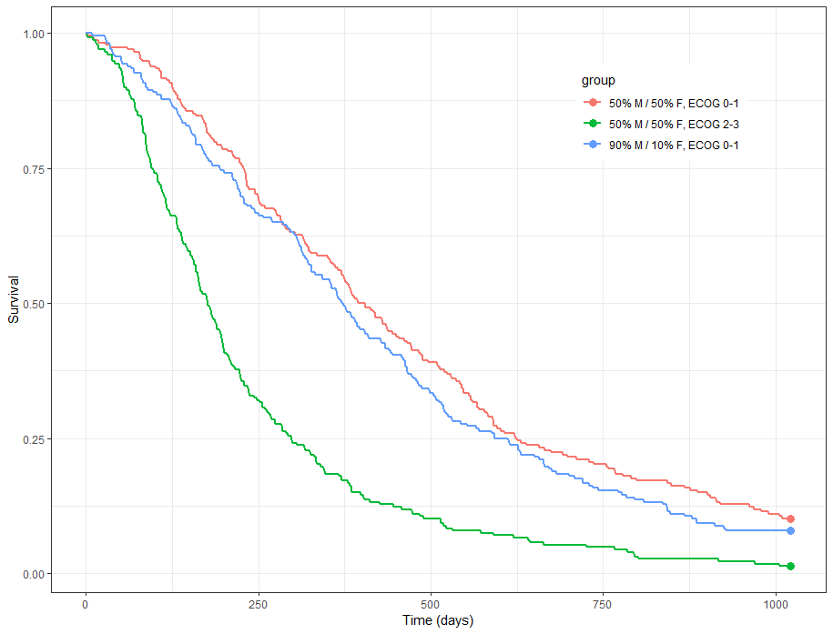
group.labels <- c("50% M/50% F, ECOG 0-1", "50% M/ 50% F, ECOG 2-3","90% M/10% F, ECOG 0-1" )
kmplotmlx(EvRes,labels=group.labels,facet=FALSE) + xlab("Time (days)") + ylab("Survival") +
theme(legend.justification=c(1,1), legend.position=c(0.9,0.9))
We obtain the following prediction:
 Because the time of death is a random variable, several simulations of the same population will lead to different survival curves. We can assess the uncertainty of the survival curve by doing replicates. This can be done very easily by adding an argument nrep:
res1 <- simulx(project = project.file,
               parameter = cov1,
               nrep = 100)
We then obtain a prediction interval for the three survival curves: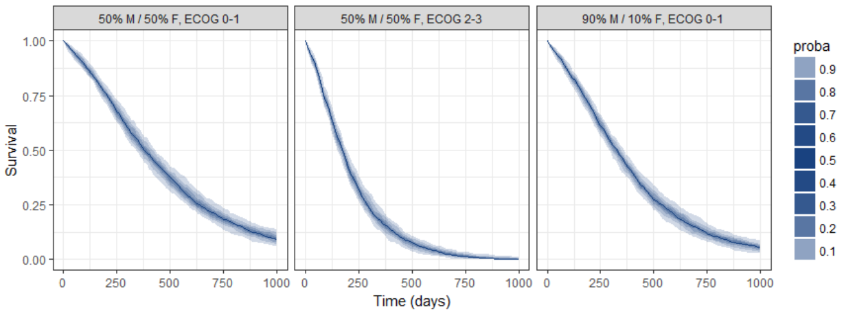
Conclusion
The MonolixSuite is a powerful tool for modeling and simulation of time-to-event data via a parametric approach. Covariates, frailty models and censoring can easily be incorporated. Build-in statistical tests and diagnostic plots (in particular the “visual predictive check for TTE data”) render the model development process straightforward.
With the lung cancer data set of this case study, the risk of death increases over time (Gompertz distribution of death times). Sex and the ECOG performance score are significant covariates and thus prognostic factors. Performance scores assessed by patients rather than physicians can also serve as prognostic factors but their utility in addition to the physicians measured score is small.
Thank to the parametric formulation of the model, survival probabilities depending on the sex and ECOG score can easily be computed. In addition, simulations of cohorts with combination of covariates can be performed using Simulx and the uncertainty of the resulting survival curve can be visualized.