Vanoxerine C-QTc case study

Sudden cardiac death is among the most common types of mortality in developed countries and accounts for 50% of all cardiovascular based deaths. Of this 50%, 80-85% is caused by acute ventricular arrhythmia, which can be triggered by prolongation of the ventricular re-polarization, or in other words, prolongation of the QT interval.

The QT interval is measured on an electrocardiogram and describes some of the electrical properties of the heart. It is a time from the start of the Q wave to the end of the T wave and approximates the time between a moment when cardiac ventricles start to contract and when they finish relaxing. An abnormally long QT interval may result in early after depolarization (EAD), which may provoke torsade de pointes and fatal ventricular arrhythmia [R.F. Jr. Gilmour et al. (1997)]. Causes of this behavior can be genetic, pathological, due to other diseases such as diabetes or rheumatoid arthritis. But, it can be also associated with adverse drug reactions. This case study is dedicated to the latter case, in which the main objective is to asses the risk of a drug on a cardiovascular safety. Two approaches can be distinguished:

Thorough QT (TQT) study is a dose-effect analysis with discrete measure. The aim is to determine if a drug has a threshold effect on cardiac re-polarization detected by the QT interval prolongation. According to guidelines, the threshold cannot be crossed at any time point after administration of a drug in order to accept it. This can lead to a strong bias and false negative results. [E14 Guideline (2005)]
Concentration-QT (C-QT) study is a continuous measure approach and describes the concentration-effect relationship. Using data from all doses and time points, the PKPD framework can provide an insight to help in decision process [Ch. Garnett et al. (2017)], [N.P. France and O. Della Pasqua (2015)].

Studies of the relationship between a drug concentration and the QT interval have successfully assessed drug induced QT interval prolongation in several known substances. Since 2005, the FDA and European regulators require analysis of a drug’s effect on the QT interval using TQT study for nearly all new molecular entities. In December 2015, the revised ICH E14 Question and Answer (R3) document enables pharmaceutical companies to use C ‐ QT modeling as the primary analysis to assess the QT prolongation risk of new drugs. But applications of PKPD modeling and simulations in the evaluation of cardiovascular safety still remain limited and face many new challenges with respect to TQT studies, for example

accuracy of the QT interval measurements and inter-studies variability [ V. Gotta et al. (2015)],
heart rate correction of the QT interval, see Section 2,
dense QT-RR data for wide range of heart rates for the baseline correction,
global vs. individual specific QT corrections [M. Malik et al. (2019)],
inter-species differences [V.F.S. Dubois et al. (2016)],
choice of a dependent variable in PKPD models [P. Dalong et al. (2018)].

This case study, based on the example of Vanoxerine, presents a possible work-flow to analyze C-QTc interval relationship in the framework of population PKPD modeling using MonolixSuite applications.

Data file and data exploration
Heart rate correction of the QT interval
PK model: Vanoxerine concentration
PKPD model: C-QTc interval relationship
Simulations: QTc prolongation

1. Data file and data exploration

Clinical study data

This C-QTc study workflow in Monolix is based on a clinical trial data of a human laboratory study of Vanoxerine (GBR 12909), which is 1-[2-[bis(4-fluorophenyl)methoxy]ethyl]-4-(3-phenylpropyl) piperazine dihydrochloride – a dopamine uptake inhibitor developed to treat cocaine dependence. Its human trials were blocked at Phase II because patients under treatment showed prolongation of the QT interval.

The clinical study was a single dose with escalation, double-blind trial on 15 patients, 11 males and 4 females, characterized by (mean age, std) = ( 40,3.74) and (mean weight,std) = (76.2,13.19). There were two placebo individuals, and remaining ones took Vanoxerine daily for 10 days in oral tablets. Two doses, 50mg and 75mg, where used. Drug concentration, in mg/L, was measured 12 to 22 times with an average of 19 times per patient, starting after the third dose. The QT interval measurements were obtained for patients in all arms with an average of 40 observations per patient, among which 10 measurements during one day preceding the treatment and 10 measurements during one day succeeding the treatment.

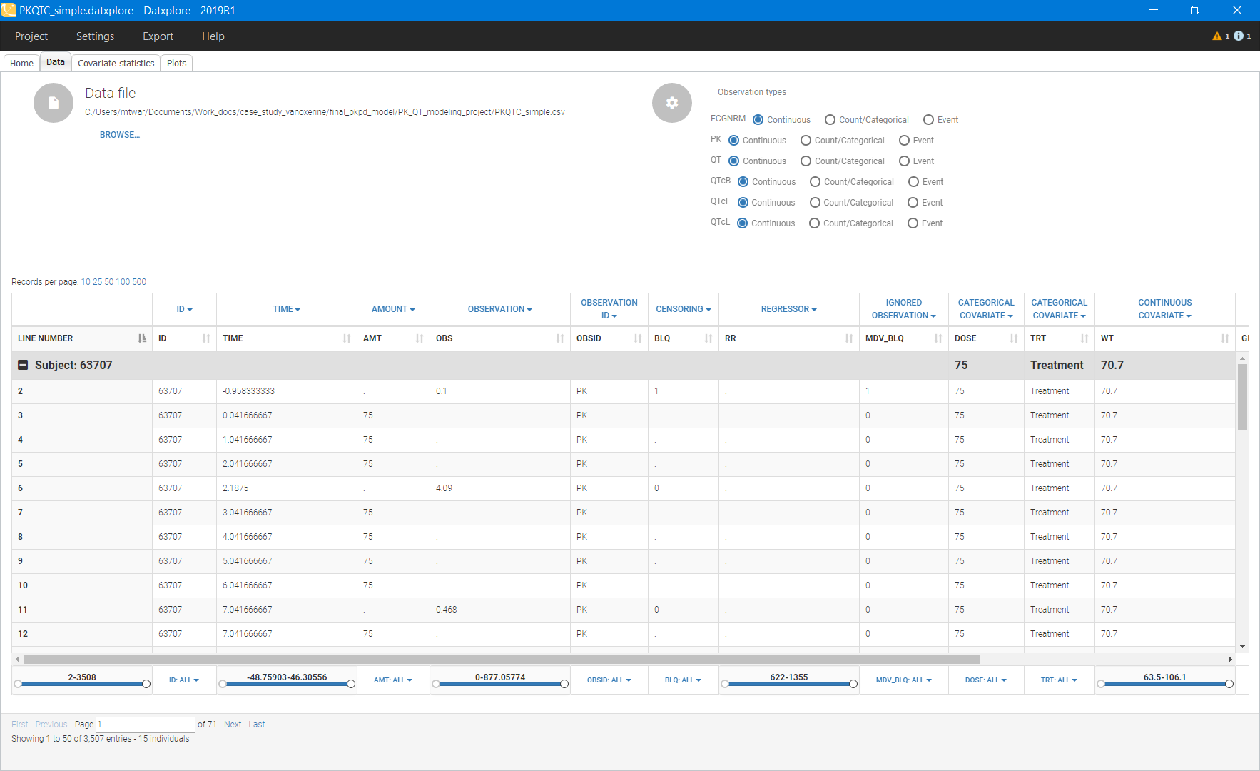
The data set csv file contains the following information:

ID: patient id number
TIME: measurement times in days
AMT: amount of administered drug in mg
OBS: measured Vanoxerine concentration in mg\mL, QT interval length in ms and corrected QTc interval using Fridericia’s formula, see Section 2
OBSID: observation ID with PK for Vanoxerine concentration, QT for interval lengths and QTc for corrected interval
RR: RR interval length in ms (used as a regressor in Monolix)
DOSE: categorical covariate: administered dose 0/50/75 mg
TRT: categorical covariate to distinguish patients with treatment and placebo
WT: continuous covariate: patient weight in kg
GENDER: categorical covariate: 1 – male, 2 – female
AGE: continuous covariate: patients age in years
PLACEBO: categorical covariate: 1 – placebo, 0 – treatment

Below is an extract of the data set file opened in Datxplore:

Data exploration

Datxplore visualizes the data set and gives the first insight into the features of the structural and statistical model.

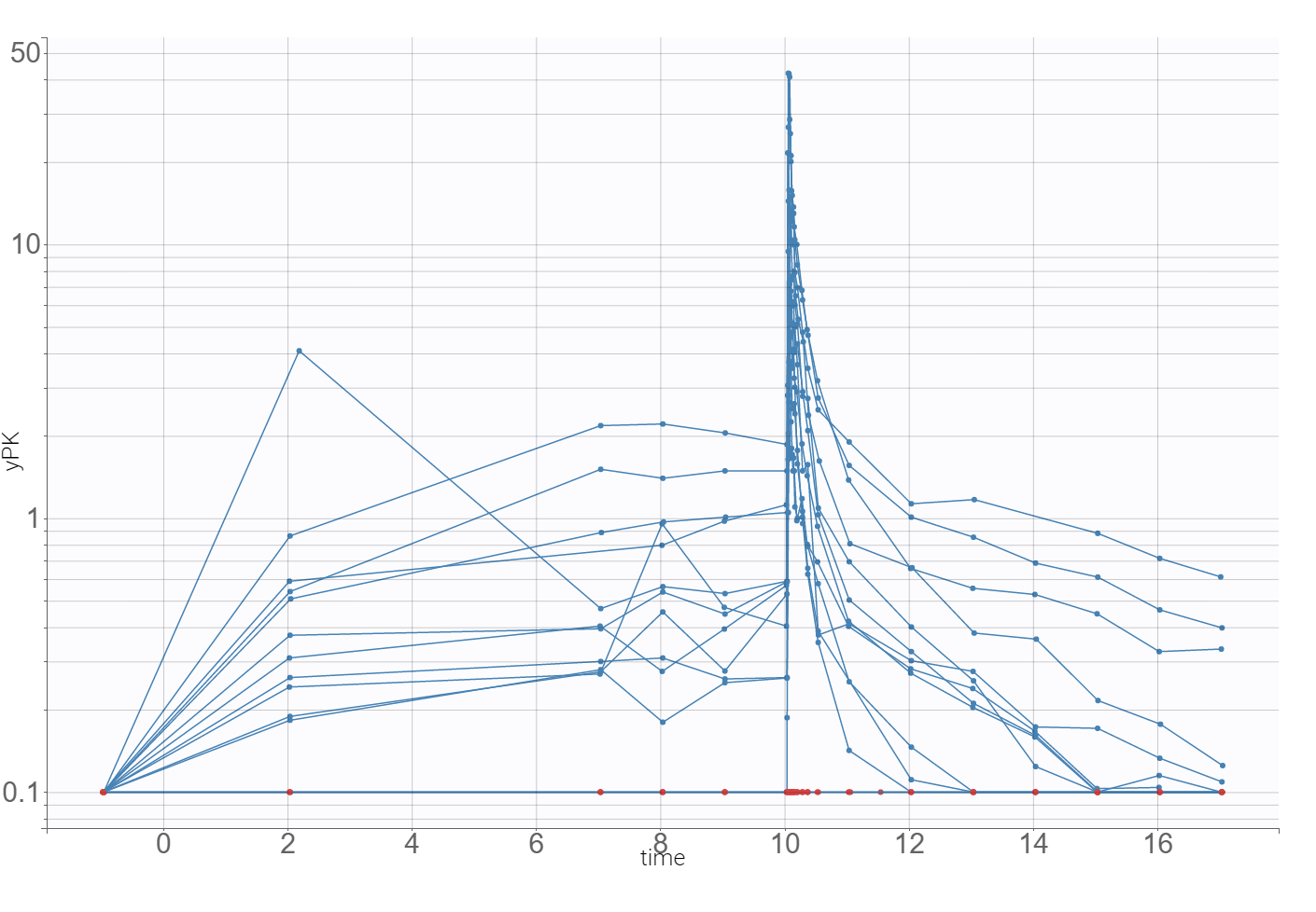
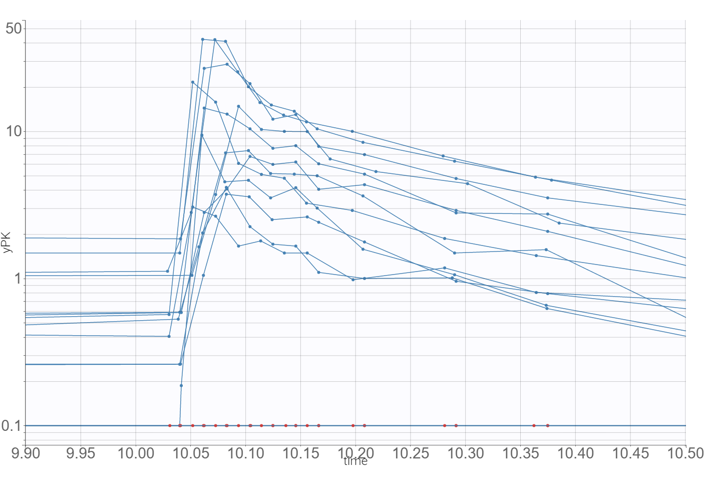
The time evolution of the drug concentrations, presented below on the left with the log-scale on the y-axis, shows that a PK model needs at least two-compartments to describe the elimination phase. A delay in the absorption can explain a shift in the location of the maximal concentration with respect to the last dose (at time=10), which is observed in the zoomed plot on the right.

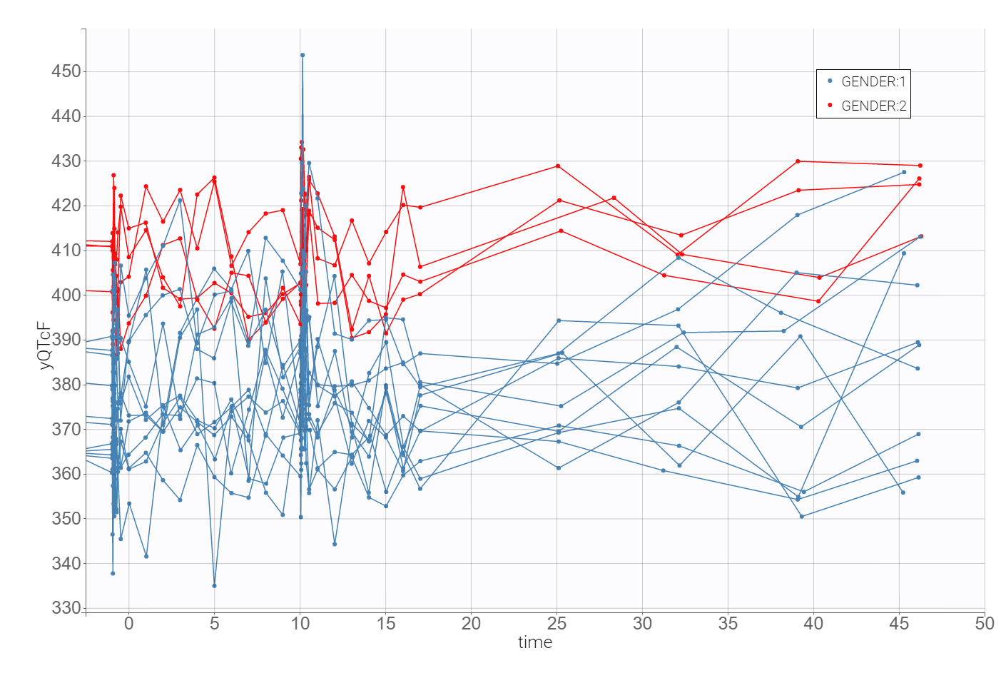
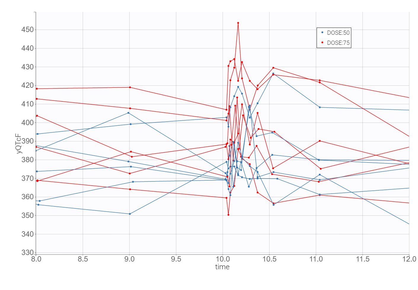
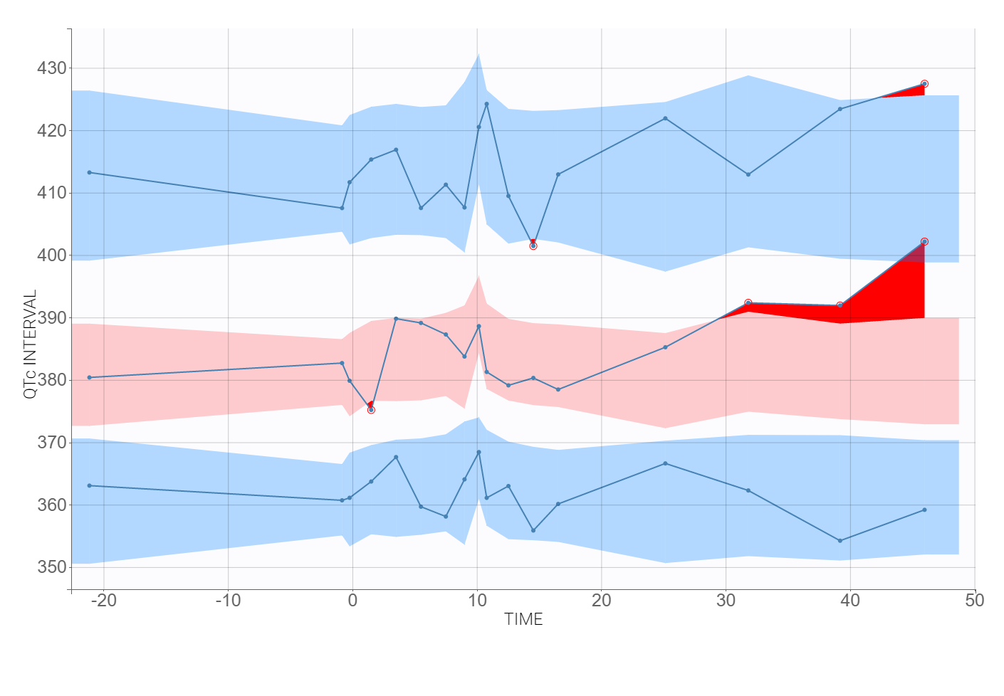
The time evolution of the heart rate corrected QTc interval, displayed below on the left, contains a stratification by gender. This covariate explains some of the variability in the QT baseline value – higher for females. The length of the QT interval increases after the treatment, shown on a zoomed image on the right, but the relationship between the dose amount/concentration and the QT interval prolongation cannot be easily deduced from these observations.

2. Heart rate correction of the QT interval

Heart rate affects the QT interval and it is undesirable in the C-QTc analysis. The heart-rate corrected QT interval (QTc), that is the QT interval converted to a value that would be expected if its HR was constant, can be obtained by various formulas. They are derived from QT-RR pairs collected by ECG recordings. Among three main approaches, two give one correction to all individuals, and one takes into account the variability between them.

Methods

General method derived from a historical population. This method is based on ECG recordings of normal, healthy volunteers in the past and is usually sufficient if the medicine does not have an effect on the heart rate. The most well-known and clinically used are the Bazett’s formula (QTcB) [H.C. Bazett (1920)] and the Fridericia’s formula (QTcF) [L.S. Fridericia (1920)] . They are parabolic corrections based on the assumption that QT and RR intervals are log-normally distributed and use the power law

$QTc = QT\cdot \left(\frac{RR}{(1s)}\right)^{-\alpha},$

with the coefficient $\alpha = 1/2$ or $\alpha = 1/3$ for the Bazett’s and the Fridericia’a method respectively. The QT interval is in mili-seconds and the RR interval in seconds, with

$RR [s] = \left(\frac{HR[\textrm{beats-per-minute}]}{60}\right)^{-1}.$

Bazett’s formula under-corrects at faster heart rates (over 60 bpm) and conversely over-corrects at slower heart rates, so the Fridericia’s formula became a standard method for calculating the hear rate corrected QTc interval.
General method derived from the population under study. This method uses off-treatment data of individuals that participate in a clinical trial and constructs a general formula according to Bazett or Fridericia approach.
Specific method derived for each individual in the population under study. It is an individual-specific correction that requires the QT-RR data for a wide range of heart rates for each individual during off-treatment conditions. Assuming the log-normal distribution of QT-RR pairs, as for the Fridericia’s formula, the model writes as [V. Piotrovsky (2005)]

$QT_{ij} = QTc0_i (1+CIRC_{ij}) \cdot RR_{ij}^{\alpha_i}$

for all $i=1,...,N$ at times $t_j, j=1,...,J_i$ .

The term CIRC corresponds to the circadian rhythm, which drives the daily variability of heart rate, and is modeled by an oscillatory function, for example by phasor functions,

$CIRC = \sum_{l=1}^{L} A_l \cos\left(\frac{2\pi}{\omega_l}(t-\phi_l)\right).$

Recent research [M.Malik et al. (2019)] on the performance of individual-specific and general corrections shows a high bias in the population/general parameter estimates and points out the necessity of dense intra-subject QT-RR to derive reliable subject-specific corrections.

Note: The heart-rate correction is necessary to perform accurate C-QT analysis. Other factors, such as gender, weight, age or food intake, also influence the length of the QT interval. They can explain the variability between individuals and work in a model as covariates.

Remark: Another feature that influence the quality of the QT correction is the QT-RR hysteresis. It describes how quickly the QT interval changes when heart rate changes. In healthy subjects it takes at least 2 min for the QT interval duration to stabilize after an abrupt heart rate change [C.P. Lau (1988)]. To account for the hysteresis effect a sequence, at times $\delta t =\{t_{j},t_{j+1},...,t_{j+\bar{k}}\}$ , of the RR interval measurements is needed for each QT correction, that is $\left\{RR_{ij}^{k}\right\}_{k=0}^{\bar{k}}$ , where $RR_{ij}^0$ is the measurement at time $t_{j}$ [M. Malik et al. (2018)]. Then, the exponential-decay hysteresis correction uses

$RR'_{ij} = \sum_{k=0}^{\bar{k}} \omega_{k} RR_{ij}^{k}$

to correct the QT interval. Omission of QT-RR hysteresis increases the variability of the QTc data and may increase the confidence intervals of the estimates of a drug-induced QTc prolongation.

Individual-specific QT interval correction using the Vanoxerine data set

The aim is to assess if the individual-specific approach to obtain heart rate corrected QT interval using the Vanoxerine data set is better then general formulas such as Bazett’s and Fridericia’s. The data set is not very dense and two structural models are considered: with and without the circadian rhythm. The models are respectively

$QT_{ij} = QTc0_i\left[(1+A_i\cos\left(\frac{2\pi(24t-\varphi)}{24}\right)\right]\left(\frac{RR_{ij}}{1000}\right)^{\alpha}$

and

$QT_{ij} = QTc0_i\left(\frac{RR_{ij}}{1000}\right)^{\alpha},$

where QTc0, A, $\varphi$ and $\alpha$ are individualized parameters, time t is given in days and RR in ms.
The model written in the Mlxtran language is:

[LONGITUDINAL] input = {qtc, alpha, RR} RR = { use = regressor } EQUATION: QT = qtc*(RR/1000)^(alpha) outRR = RR OUTPUT: output = {QT}

To parametrize the model, Monolix uses all QT-RR measurements for the placebo patients, and only drug-free QT-RR measurements for patients on the drug, during one day prior to the treatment. The sparse data set makes it difficult to find good initial estimates, so the SAEM algorithm is initialized with all parameters equal to 1. The following table presents the comparison of different models in Sycomore:

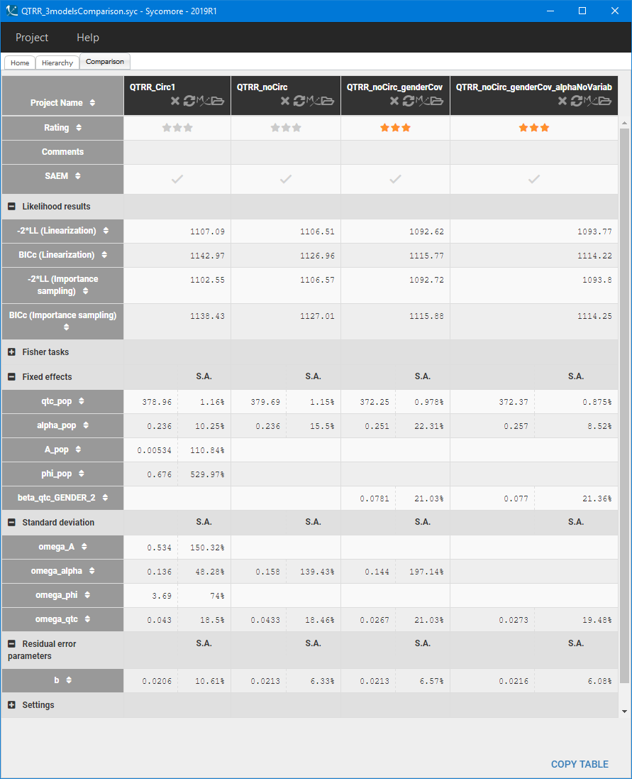
The first two columns compare the population parameters, standard deviations and likelihood results of the two structural models. Standard deviations of the circadian rhythm parameters are very high and the estimated value of the amplitude A is of order $10^{-3}$ , compared to $QT\sim 10^3$ . Model neglecting the circadian rhythm has better BICc criterion, despite the fact that the accuracy in estimating $\alpha$ and $\omega_{\alpha}$ decreased, and is chosen as the final structural model.

For the statistical model, the Pearson’s correlation tests indicate that gender is significantly correlated with QTc0. It explains part of the variability of QTc0, which is consistent with the biological characteristics – females have longer QT interval then males – and with the initial data exploration. Adding gender as a covariate effect on the QTc0 improves the BICc value of the model (third column in the Sycomore table above), but at the same time worsens again the accuracy of $\alpha$ . Removing the inter-individual variability of $\alpha$ does not change significantly the value of BICc and parameter estimates (last column in the Sycomore table above). This model is close to the general approach, such as Fridericia’s formula, where one value is used for all individuals. The coefficient $\alpha_{pop}=0.257$ is smaller than the Fridericia’s coefficient and, as shown below, the QTc interval is less dependent on RR.

But full QT-RR off-drug profiles are not available for the Vanoxerine data set, and individual-specific approach can be biased [M. Malik et al. (2019)]. To avoid this, the Fridericia’s formula $\alpha=1/3$ defines the corrected QTc interval in model developed in Section 4.

R-code

Below is the code to generate the plots. The QTc-RR model contains regressor (RR interval), so the Monolix Project has to be first converted into an executable R script for the simulator Simulx, by running the following lines:

#generation of an executable R script from the Monolix project
setwd("path to your project mlxtran file")
monolix2simulx("your_project_name.mlxtran")

It creates a folder “your_project_name_simulx” with the executable R code for simulx and the data files used for the simulation (parameters, observation design, dosage regimen, covariates). The following modifications directly in the R-script allow to produce the QTc-RR plots:

setwd("path to the your_project_name_simulx folder")
# model
model <- "your_project_name_simulxModel.txt"

# parameters
originalId <- read.csv('originalId.txt')
populationParameter <- read.vector('populationParameter.txt')
colCatType <- rep(NA,7)
catNamesCols <- c(4,5,6,7)
colCatType[catNamesCols] <- rep("character",4)
individualCovariate <- lixoft.read.table(file='individualCovariate.txt', header = TRUE, colClasses = colCatType)
individualCovariate[,4] <- as.factor(individualCovariate[,4])
individualCovariate[,5] <- as.factor(individualCovariate[,5])
individualCovariate[,6] <- as.factor(individualCovariate[,6])
individualCovariate[,7] <- as.factor(individualCovariate[,7])
list.param <- list(populationParameter,individualCovariate)

# output
time <- read.csv("output.txt",header=TRUE, sep=',')
out1 <- list(name="y1",time=time)
out2 <- list(name="QT",time=time)
out3 <- list(name="alpha")
out4 <- list(name="outRR",time=time)
out  <- list(out1,out2,out3,out4)

# regressor
regressor <- read.csv("regressor.txt",stringsAsFactors=FALSE)

# call the simulator
res <- simulx(model=model,parameter=list.param,output=out,regressor=regressor)

# Replicate indyvidual parameters
nb_ids <- data.frame(table(res$QT$id))
alpha_id <- rep(res$parameter$alpha,nb_ids$Freq)

# define heart rate corrected QTc
QT_data <- read.csv("output.txt",header=TRUE, sep=',')
QT_data$RR <- res$outRR$outRR/1000
QT_data$QTc_ind <- QT_data$y1/QT_data$RR^(alpha_id)
QT_data$QTc_F <- QT_data$y1/QT_data$RR^(1/3)
QT_data$QTc_B <- QT_data$y1/QT_data$RR^(1/2)

# generate plots
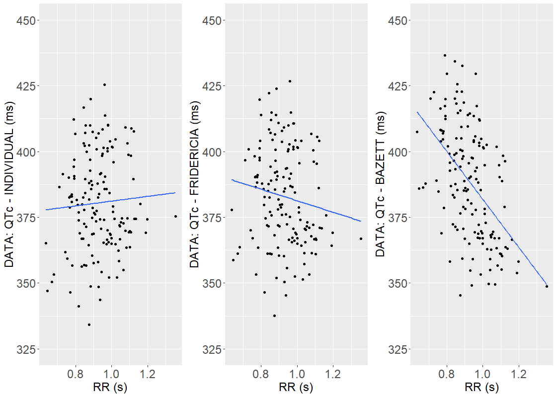
plot1 <- ggplot(data=QT_data, aes(x=QT_data$RR, y=QT_data$QTc_ind)) + ylim(325,450) + geom_point() + geom_smooth(method = "lm", se = FALSE)
                   theme(axis.text = element_text(size=18), axis.title=element_text(size=18)) +
                   xlab("RR INTERVAL (s)") + ylab("DATA: QTc - INDIVIDUAL (ms)") 
plot2 <- ggplot(data=QT_data, aes(x=QT_data$RR, y=QT_data$QTc_F))+ ylim(325,450) + geom_point() + geom_smooth(method = "lm", se = FALSE)
                   theme(axis.text = element_text(size=18),axis.title=element_text(size=18)) +
                   xlab("RR INTERVAL(s)") + ylab("Data: QTc - FRIDERICIA (ms)") 
plot3 <- ggplot(data=QT_data, aes(x=QT_data$RR, y=QT_data$QTc_B))+ ylim(325,450) + geom_point() + geom_smooth(method = "lm", se = FALSE)
                   theme(axis.text = element_text(size=18),axis.title=element_text(size=18))
                   xlab("RR INTERVAL(s)") + ylab("Data: QTc - BAZETT (ms)")
grid.arrange(plot1, plot2, plot3, ncol = 3)

3. PK model: Vanoxerine concentration

Structural model

Visualization of the time evolution of Vanoxerine concentration in Section 1, indicated that a PK model requires at least two compartments to describe the elimination process. A base structural model with two-compartments, a 1-st order absorption and a linear elimination rate is chosen from the Monolix PK library:

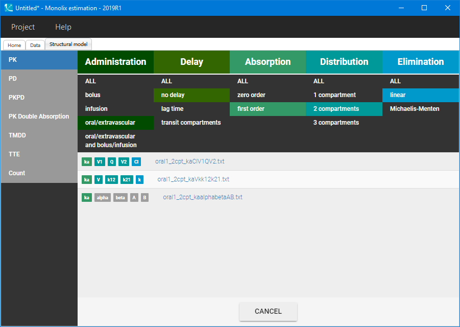
Then, the “Auto-init” function initializes the parameters for the SAEM algorithm, and gives the following examples of the initial distributions:

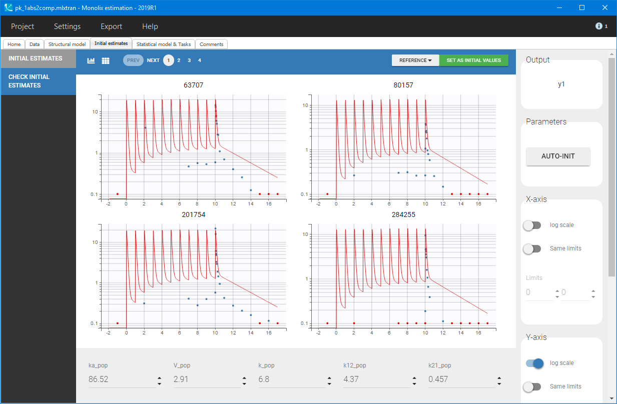
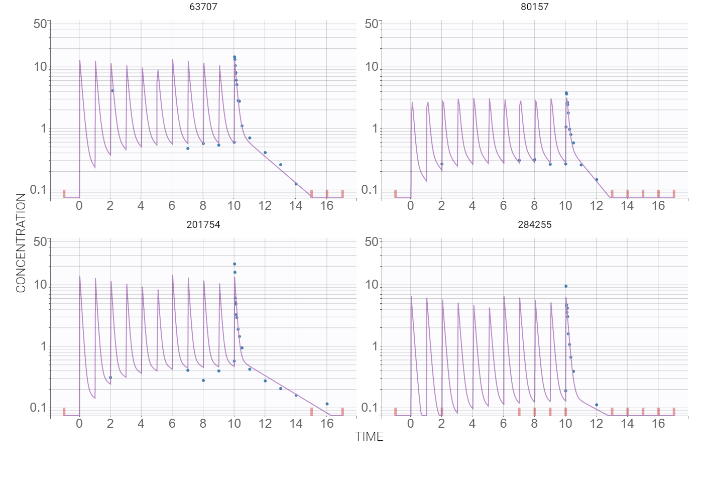
At this stage, the default error and statistical models settings are kept – combined error, no covariates and no correlations – and Monolix tasks are lunched after saving the project. The model individual fits, presented below for several individuals, are satisfactory.

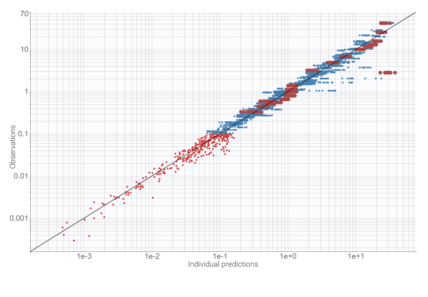
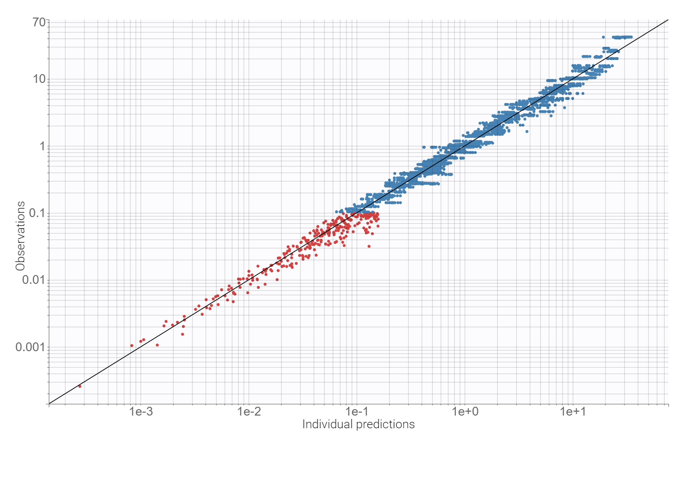
Observation vs. predictions diagnostic plot, obtained using the individual estimates from the conditional distribution and shown below, has outliers at measurements just after the last dose. This suggests a possible delay in the absorption. Additionally, the value of the additive parameter of the error model, available in the “Results” tab, is of order $10^{-4}$ , compared to concentration levels between 0-20, so a proportional model is sufficient.

Adding a lag time to the absorption and using the proportional error model improves the BICc criterion by approximately 10%. There are no more mis-specifications in the observation vs. predictions plot:

Finally, a convergence assessment shows that the convergence of the SAEM algorithm is robust with respect to different initial estimates of the population parameters.

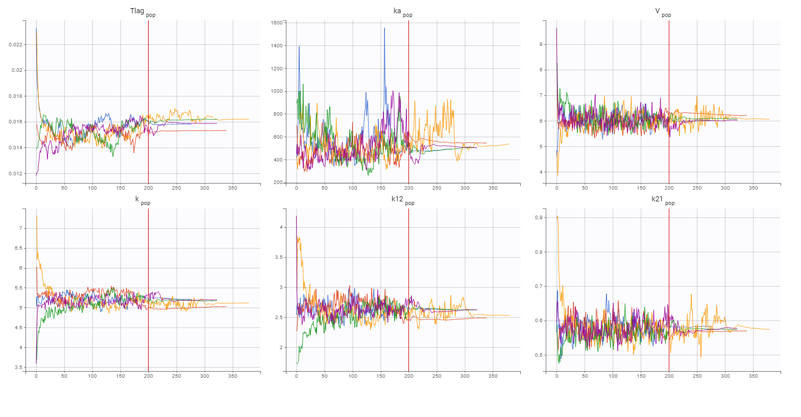
Statistical model

Diagnostic plots and statistical tests provided by Monolix help to explain the model variability. High p-values of Pearson’s correlation tests indicate weak correlations between covariates and individual parameters. But significant correlations between all three parameters V, k and k21 are observed in the following diagnostic plots:

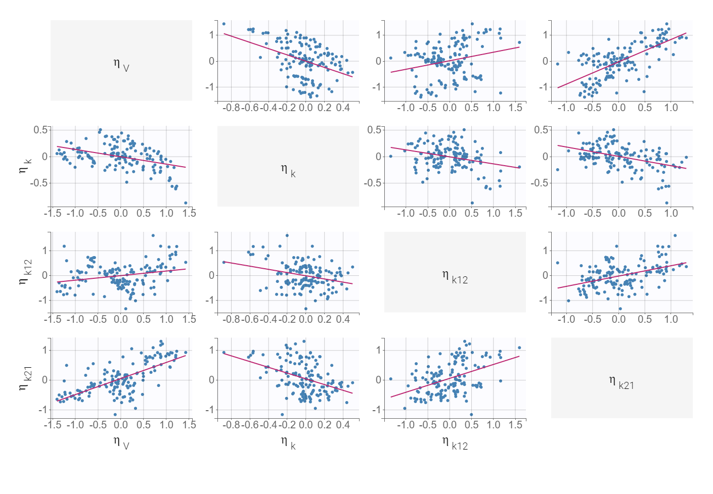
The correlation between V and k21 is stronger then between V and k.Examination of all possibilities showed that adding only the (V,k21) correlation gives the best BICc value. The model development is compared in Sycomore:

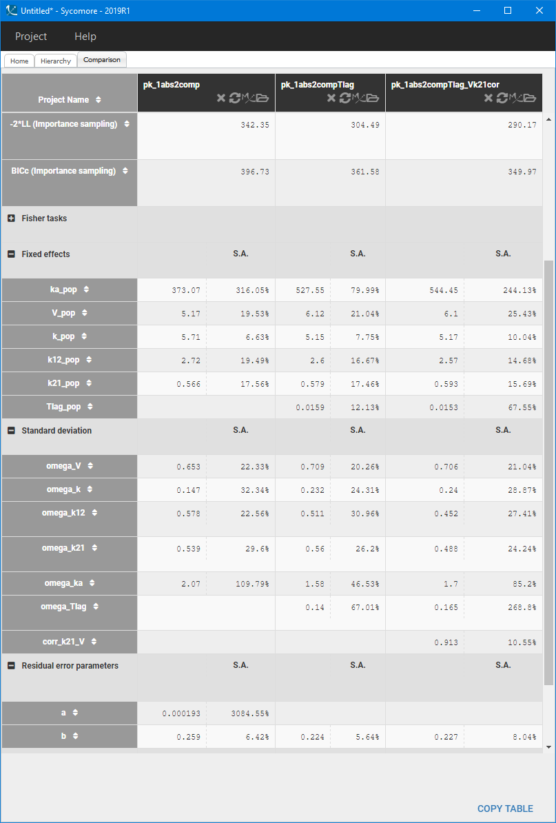
The VPC for the final model, with a lag time and a correlation between V and k21, is:

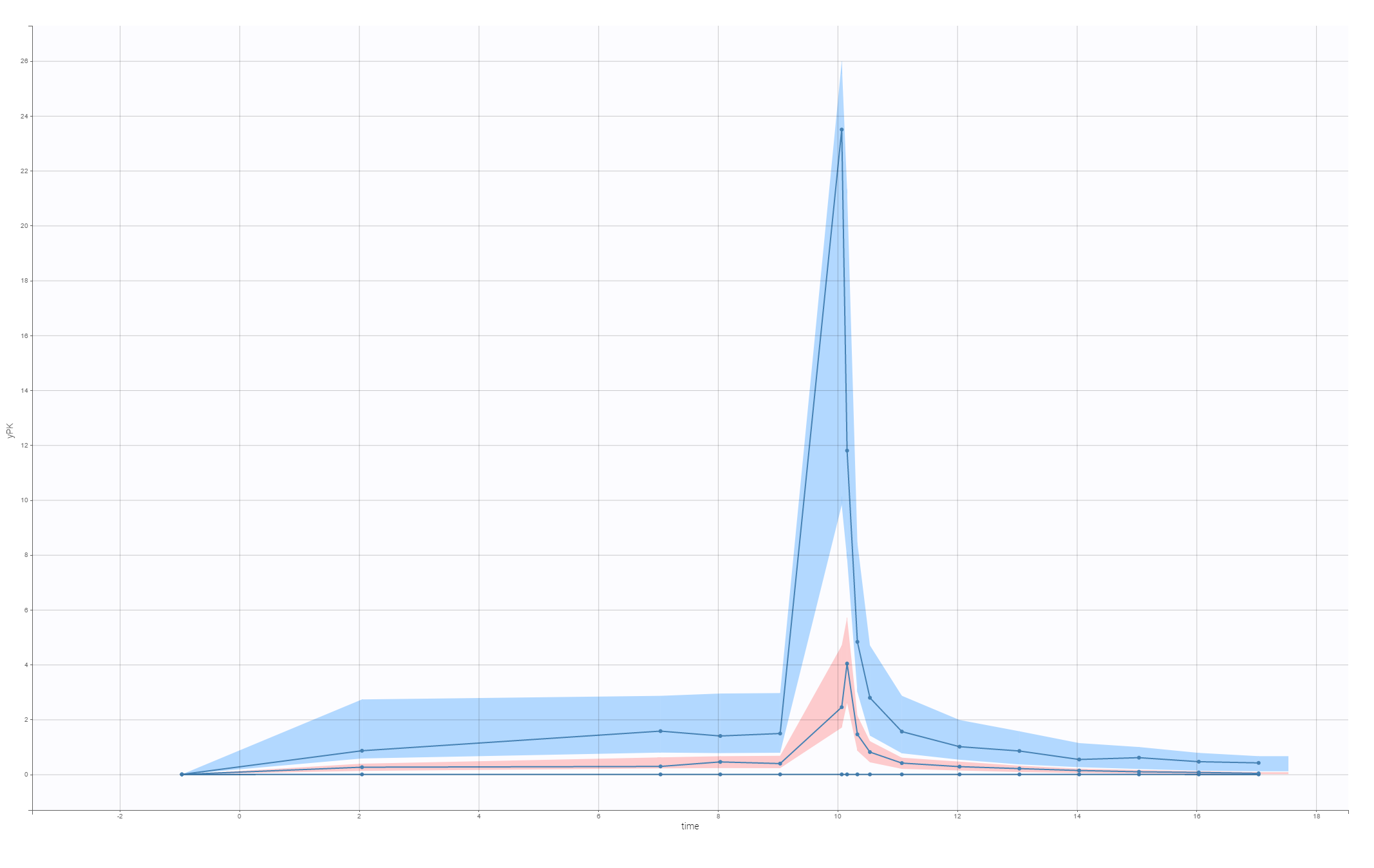
This model is used to develop PKPD model for the C-QT analysis.

4. PKPD model: C-QTc interval relationship

Heart rate corrected QTc interval is required to develop a PK-PD model for the C-QTc study. Analysis in Section 2 showed that the individual-specific QT-RR model is superior to the Fridericia formula for the Vanoxerine data set. But the quality of the data set makes the results unreliable and the Fridericia coefficient is chosen to obtain the corrected QTc interval

$QTc_{ij} = QT_{ij}RR_{ij}^{-1/3}.$

This C-QTc study uses measurements at all time points, before and after the treatment, which differs from the QT-RR relationship analysis, where only before-treatment points were taken into account.

C-QTc model

The aim of a C-QTc model is to compute the placebo adjusted change of the QTc interval from the baseline, denoted by $\Delta\Delta QTc$ . It is defined for all individuals and represents the difference between a model-derived, baseline corrected QTc interval at a concentration of interest during a treatment $\Delta QTc^{\textrm{trt}}$ and a model-derived, baseline corrected QTc interval in the placebo case (concentration=0) $\Delta QTc^{\textrm{plc}}$ :

$\langle\Delta\Delta QTc(C)\rangle = \langle\Delta QTc_{i}^{trt} (C_{ij})\rangle - \langle\Delta QTc_{i}^{plc}(0)\rangle,$

where $\langle\cdot\rangle$ is an estimated mean [Ch. Garnett (2017)]. The baseline correction $\Delta QTc = QTc - QTc0$ is usually chosen as a dependent variable of a model and is obtained from a collection of the QT data over a wide range of heart rates on the day before the treatment. In this case study, the density of the on- and off-treatment ECG measurements is insufficient for this approach and the dependent variable is directly the QTc interval length, which requires assumptions on the effect E of a drug on the QT interval.

A basic population PKPD model is composed of three terms:

$QTc_i = QTc_{0i} + CIRC_i + E_i(C),$

where

QTc0 is the intercept – individual corrected baseline QTc in the absence of treatment,
CIRC is an oscillatory function accounting for the circadian rhythm,
E is a drug effect assumed to have linear or Hill type form

$E = E0\cdot C, \qquad E = E\textrm{max} \frac{C}{{EC50}+C},$

with E0 – a linear rate, EC50 – a concentration at which the effect is half of its maximum Emax,
C is the concentration of a drug in plasma or in effect compartment predicted by a population PK model. It can be calculated separately or, as in this case study, together with the PD model.

Monolix estimates the parameters of the C-QTc model. They are used to calculate the placebo adjusted change of the QTc interval from the baseline at a concentration of interest defined as $\Delta\Delta QTc(C) = E(C)$ .

Remark: To include an individual heart rate correction of the QT interval, the model should be transformed to

$QT_i = QTc_{0i} RR^{\alpha_i} + CIRC_{i} + E_i(C),$

where the RR interval is classified as a regressor in Monolix.

Vanoxerine effect: model development

The PK model describing the Vanoxerine concentration was developed in Section 3. A two compartment model with the 1st order absorption, a time lag and a linear elimination, parametrized by (Tlag,V,ka,k,k12,k21) and including V-k21 correlation gives the best fit. The PD part of the model describes the effect E of a drug and, in this case study, represents directly the prolongation of the QT-interval.

The following structural PKPD models without the circadian rhythm and with a default statistical model are compared

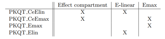
Table below shows the results of Monolix tasks using Sycomore:

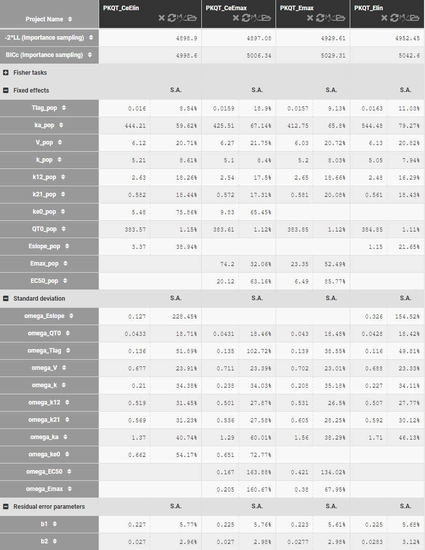
Model development starts with a C-QT model with nighter the circadian rhythm nor the effect-comportment. Estimates of the model parameters and standard deviations, shown above, are comparable for linear and Emax response function, but the BICc criterion is lower in the former case. It can be caused by the quality of the data set, which is not dense enough to estimate correctly all parameters of the Emax function. The estimates of the EC50 concentration are relatively large with respect to the drug’s concentration (C<20mg/L), which explains further the superiority of the linear response. Adding the effect compartment improves the fits in both cases. The circadian rhythm influences the QT-interval and should be added to the model, but this term cannot be correctly estimated using this data set. For example, using the simplest phasor function,

$CIRC=A\cos(2\pi(t-\varphi)),$

the estimated amplitude is of order $10^{-4}$ and the standard deviation of the phase is above 500%.
The model written in the Mlxtran language is:

[LONGITUDINAL] input = {Tlag, ka, V, k, k12, k21, ke0, QT0, E0} EQUATION: ;====== PK part of the model {Cc,Ce} = pkmodel(Tlag, ka, ke0, V, k, k12, k21) ;====== PD part of the model E = E0*max(Ce,0) QTc = QT0 + E OUTPUT: output = {Cc,QTc}

For the Emax response function the input has two PD parameters: Emax, EC50 (instead of E0) and the response is defined as E=Emax*max(Ce,0)/(EC50+max(Ce,0)).

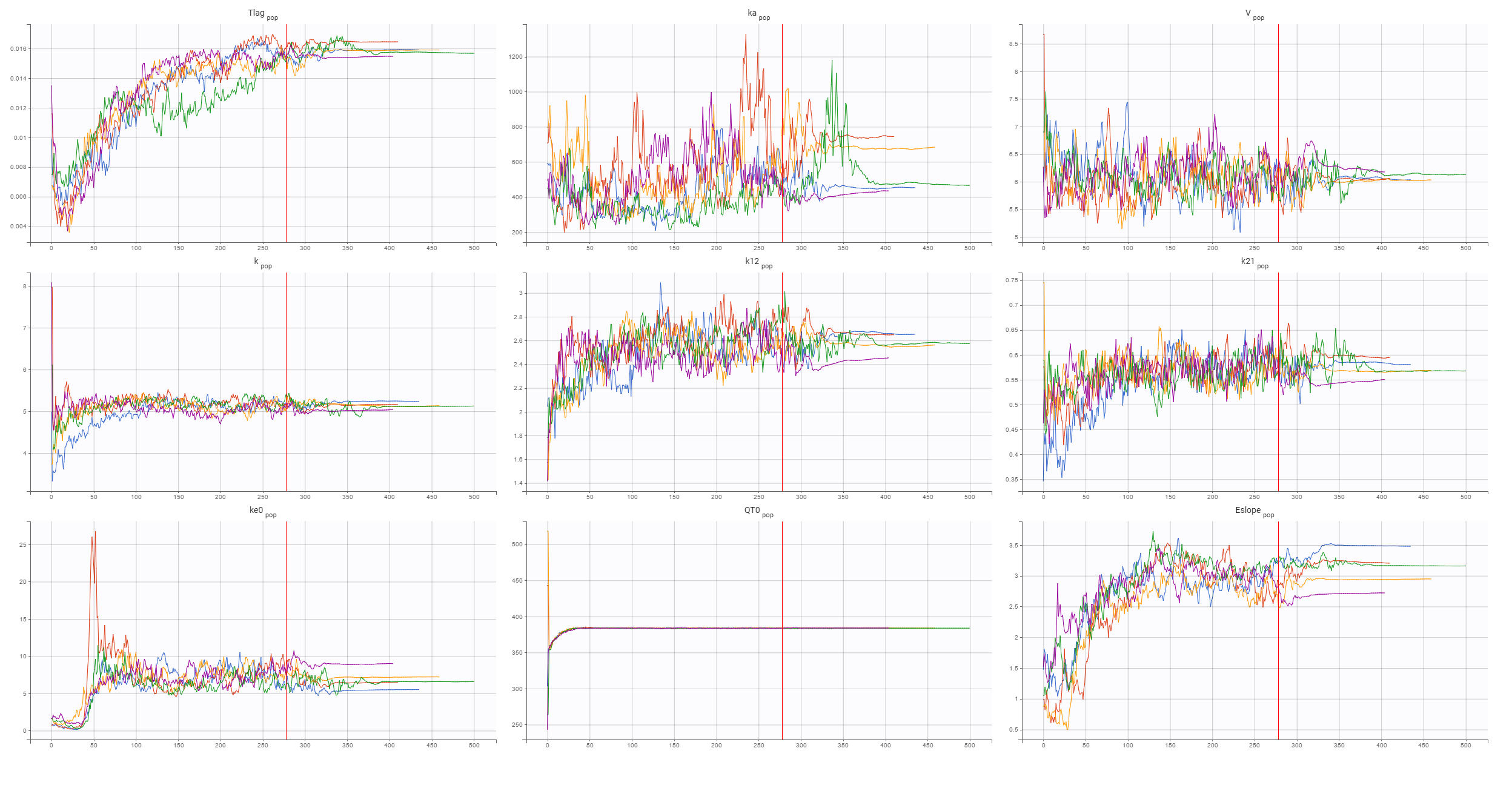
The final structural PD model for the C-QTc relationship is a linear response model with an effect compartment. The convergence of the SAEM algorithm, shown below, confirms reliability of the estimates:

Now, the statistical model can be analyzed. As in the case of QT-RR study, gender explains part of the variability of the baseline QTc0 and, together with the (V,k21) correlation, improves the BICc criterion. Despite the high variability in the data, observed in the individual plots below

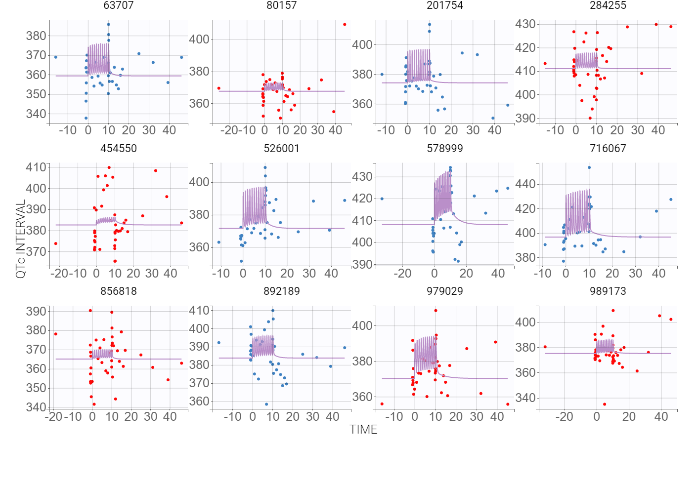
the VPC plot confirms that this PKPD model can be estimated with quite good confidence.

5. Simulations: drug induced QTc prolongation

The aim of the C-QTc analysis is to asses the risk that a new drug induces a prolongation of the QTc interval. In other words, how $\Delta\Delta QTc$ changes after administrating the drug. A guideline criterion, given by the International Council for Harmonization revised the E14 states that:

An experimental drug is declared to have no influence on the QTc interval if the upper bound of the two-sided 90% confidence interval for model-derived $\Delta\Delta QTc$ is less then 10ms at all clinically relevant exposures.

Simulations

A C-QT model allows to analyze the effect of a drug on the QTc interval by

simulations of populations larger then in the initial data set,
simulations of scenarios with different exposures,
simulations of different doses amounts and administrations,
assessing the proportion of patients who meet the cardiac non-influence criterion.

Simulx performs simulations using the model presented in the previous section. The data set does not contain enough on- and off-treatment data to use $\Delta QTc$ as a dependent variable, so $\Delta QTc=E$ and is calculated with the parameters estimated by Monolix at any concentration of interest, see Section 4. There is also no placebo arm for each patient, so $\Delta\Delta QTc=\Delta QTc$ . The following study is preliminary and the administration of the drug is the same as in the data set – oral administration once a day during 10 days – but patients receive different amounts of a drug.

Single patient

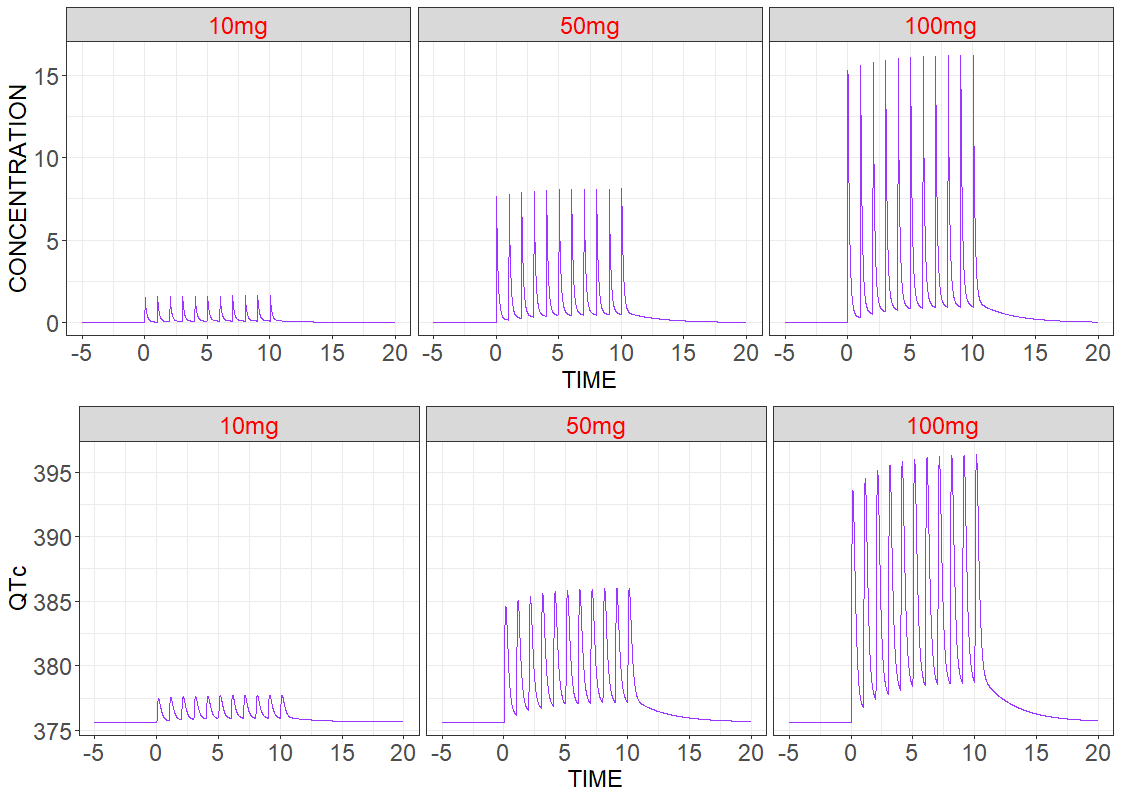
In the first simulation three patients have the same Monolix estimated population parameters without random effects, but they have different treatments – different dose amounts. Model predicted drug concentration and drug effect are presented below. As expected for Vanoxerine, the duration of the QT interval increases with the dose.

# R-script
project.file <- 'your_project_name.mlxtran'

# output
time <- seq(-5,20,by=0.01)
out1 <- list(name="Cc",time=time)
out2 <- list(name="E", time=time)

# administration
adm1 <- list(amount = 10, time=seq(0,10,by=1))
adm2 <- list(amount = 50, time=seq(0,10,by=1))
adm3 <- list(amount = 100, time=seq(0,10,by=1))

# groups: 3 patients
g1 <- list(size=1, treatment=adm1)
g2 <- list(size=1, treatment=adm2)
g3 <- list(size=1, treatment=adm3)

# set population parameters with null standard deviation
qt_dataS <- readDatamlx(project=project.file)
qt_dataS$populationParameters[grep('omega',names(qt_dataS$populationParameters))] = 0

# call the simulator
resS <- simulx(project = project.file,
               output = list(out1,out2),
               group   = list(g1,g2,g3),
               parameter=list(qt_dataS$populationParameters,c(GENDER=1)))

# generate plots
p1 <- prctilemlx(resS$Cc,label=c("10mg", "50mg", "100mg")) + theme(legend.position="none") + facet_wrap(~ group, nrow=1) + 
                 theme(strip.text = element_text(size = 18, color = "red")) + 
                 theme(axis.text = element_text(size=18), axis.title=element_text(size=18)) + xlab('TIME') + ylab('CONCENTRATION')
p2 <- prctilemlx(resS$QTc,label=c("10mg", "50mg", "100mg")) + theme(legend.position="none") + facet_wrap(~ group, nrow=1) + 
                 theme(strip.text = element_text(size = 18, color = "red")) + 
                 theme(axis.text= element_text(size=18), axis.title=element_text(size=18)) + xlab('TIME') + ylab('QTc')
grid.arrange(p1,p2, nrow=2)

Population level

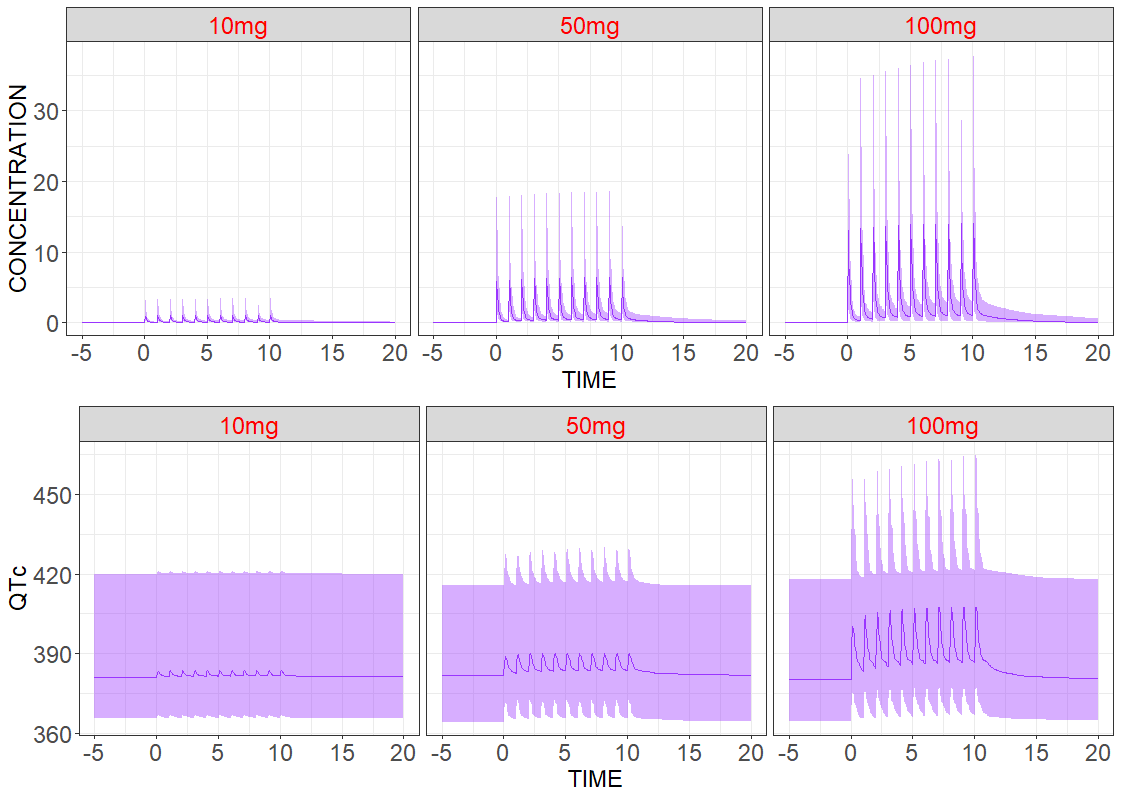
Adding inter-individual variability provides more realistic predictions among a large number of patients. As previously, three groups with different dose amounts are considered, but now the number of patients in each group is increased to N=200. Individual parameters are sampled from the conditional distribution. Median values and the 90% confidence interval of the model for the predicted drug concentration and the drug effect are the following:

# R-script
project.file <- 'your_project_name.mlxtran'

# output
time <- seq(-5,20,by=0.05)
out1 <- list(name="Cc", time=time) 
out2 <- list(name="QTc",time=time)

# administration
adm1 <- list(amount = 10,  time=seq(0,10,by=1))
adm2 <- list(amount = 50,  time=seq(0,10,by=1))
adm3 <- list(amount = 100, time=seq(0,10,by=1))

# groups
N <- 100
g1 <- list(size=N, treatment=adm1)
g2 <- list(size=N, treatment=adm2)
g3 <- list(size=N, treatment=adm3)

# call the simulator
resP <- simulx(project = project.file,
               output  = list(out1,out2),
               group   = list(g1,g2,g3))

# generate plots
p1 <- prctilemlx(resP$Cc,number=2, level=90,label=c("10mg", "50mg", "100mg")) + theme(legend.position="none") + facet_wrap(~ group, nrow=1) +
                 theme(strip.text = element_text(size = 18, color = "red")) +
                 theme(axis.text = element_text(size=18), axis.title=element_text(size=18)) + xlab('TIME') + ylab('CONCENTRATION')

p2 <- prctilemlx(resP$QTc, number=2, level=90, label=c("10mg", "50mg", "100mg")) + theme(legend.position="none") + facet_wrap(~ group, nrow=1) +
                 theme(strip.text = element_text(size = 18, color = "red")) +
                 theme(axis.text = element_text(size=18), axis.title=element_text(size=18)) + xlab('TIME') + ylab('QTc')
grid.arrange(p1,p2, nrow=2)

Drug induced QT interval prolongation: dose-effect study

An effect of a drug on the QT interval prolongation can be quantified by the change of E(C) with respect to the drug dose. The maximal increase of the QTc interval is given by E(Cmax) for the linear response function (below, on the left) and by the Emax parameter (below, on the right) for the Emax response functions

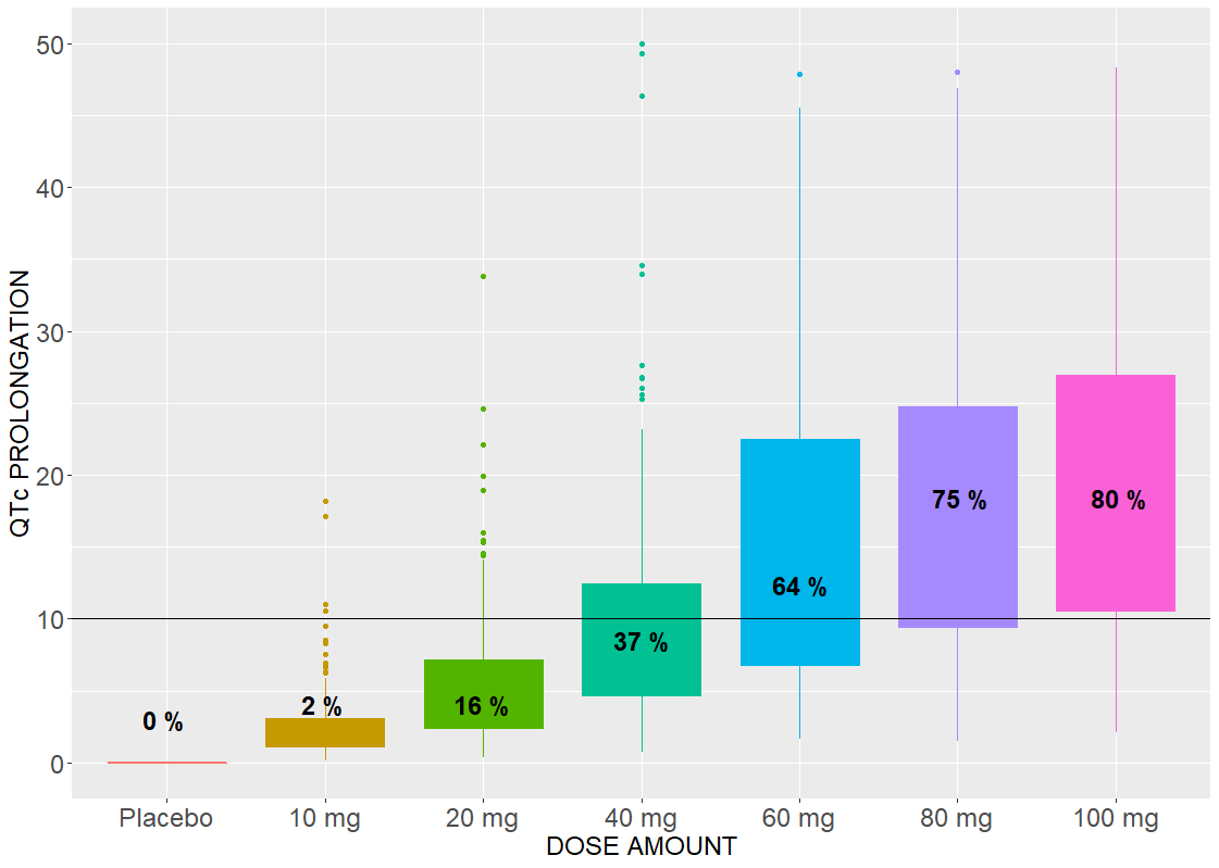
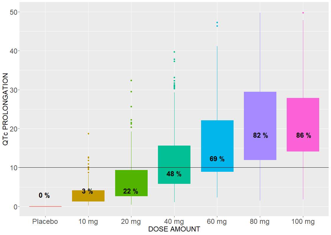
The Emax effect is interesting to compare, because simulations use higher doses than in the data. In both cases, there is a dose threshold, for which a portion of individuals suffer from the QTc prolongation.

# R-script
project.file <- 'your_project_filename.mlxtran'

# output
time <- seq(-0.1,15,by=0.05)
out <- list(name="E", time = time)

# administration
adm1 <- list(amount = 0,   time=seq(0,10,by=1))
adm2 <- list(amount = 10,  time=seq(0,10,by=1))
adm3 <- list(amount = 20,  time=seq(0,10,by=1))
adm4 <- list(amount = 40,  time=seq(0,10,by=1))
adm5 <- list(amount = 60,  time=seq(0,10,by=1))
adm6 <- list(amount = 80,  time=seq(0,10,by=1))
adm7 <- list(amount = 100, time=seq(0,10,by=1))

# groups
N < 200
g1 <- list(size=N, treatment=adm1)
g2 <- list(size=N, treatment=adm2)
g3 <- list(size=N, treatment=adm3)
g4 <- list(size=N, treatment=adm4)
g5 <- list(size=N, treatment=adm5)
g6 <- list(size=N, treatment=adm6)
g7 <- list(size=N, treatment=adm7)

# call the simulator
res <- simulx(project = project.file,
              output = list(out),
              group   = list(g1,g2,g3,g4,g5,g6,g7))

# calculate the maximal effect
dQTmax <- aggregate(res$E$E, by=list(res$E$id,res$E$group), max)

count_df <- data.frame(id=seq(1,7,by=1), prct = numeric(7)) 
for (i in seq(1,7,by=1)) {
  temp_qt <- dQTmax[dQTmax$Group.2 == i,]
  count_df[i,2] <- 100*nrow(temp_qt[temp_qt$x >=10,])/N
}

# generate plots
p <- ggplot(dQTmax, aes(x=dQTmax$Group.2, y=dQTmax$x, color = dQTmax$Group.2)) + ylim(0,50) +
               geom_boxplot(aes(fill = dQTmax$Group.2), show.legend = FALSE) +   geom_hline(yintercept=10) + 
               theme(axis.text = element_text(size=18), axis.title=element_text(size=18)) + xlab('DOSE AMOUNT') + ylab('QTc PROLONGATION') +
               scale_x_discrete(breaks=c("1","2","3","4","5","6","7"), labels=c("Placebo","10 mg", "20 mg", "40 mg", "60 mg", "80 mg", "100 mg"))

p <- p + annotation_custom(grid.text(paste(toString(round(count_df[1,2])),"%"), x=0.08,  y=0.1,  gp=gpar(col="black", fontsize=18, fontface="bold")))
p <- p + annotation_custom(grid.text(paste(toString(round(count_df[2,2])),"%"), x=0.22,  y=0.12, gp=gpar(col="black", fontsize=18, fontface="bold")))
p <- p + annotation_custom(grid.text(paste(toString(round(count_df[3,2])),"%"), x=0.36,  y=0.12, gp=gpar(col="black", fontsize=18, fontface="bold")))
p <- p + annotation_custom(grid.text(paste(toString(round(count_df[4,2])),"%"), x=0.5,   y=0.2,  gp=gpar(col="black", fontsize=18, fontface="bold")))
p <- p + annotation_custom(grid.text(paste(toString(round(count_df[5,2])),"%"), x=0.64,  y=0.27, gp=gpar(col="black", fontsize=18, fontface="bold")))
p <- p + annotation_custom(grid.text(paste(toString(round(count_df[6,2])),"%"), x=0.78,  y=0.38, gp=gpar(col="black", fontsize=18, fontface="bold")))
p <- p + annotation_custom(grid.text(paste(toString(round(count_df[7,2])),"%"), x=0.92,  y=0.38, gp=gpar(col="black", fontsize=18, fontface="bold")))
print(p)

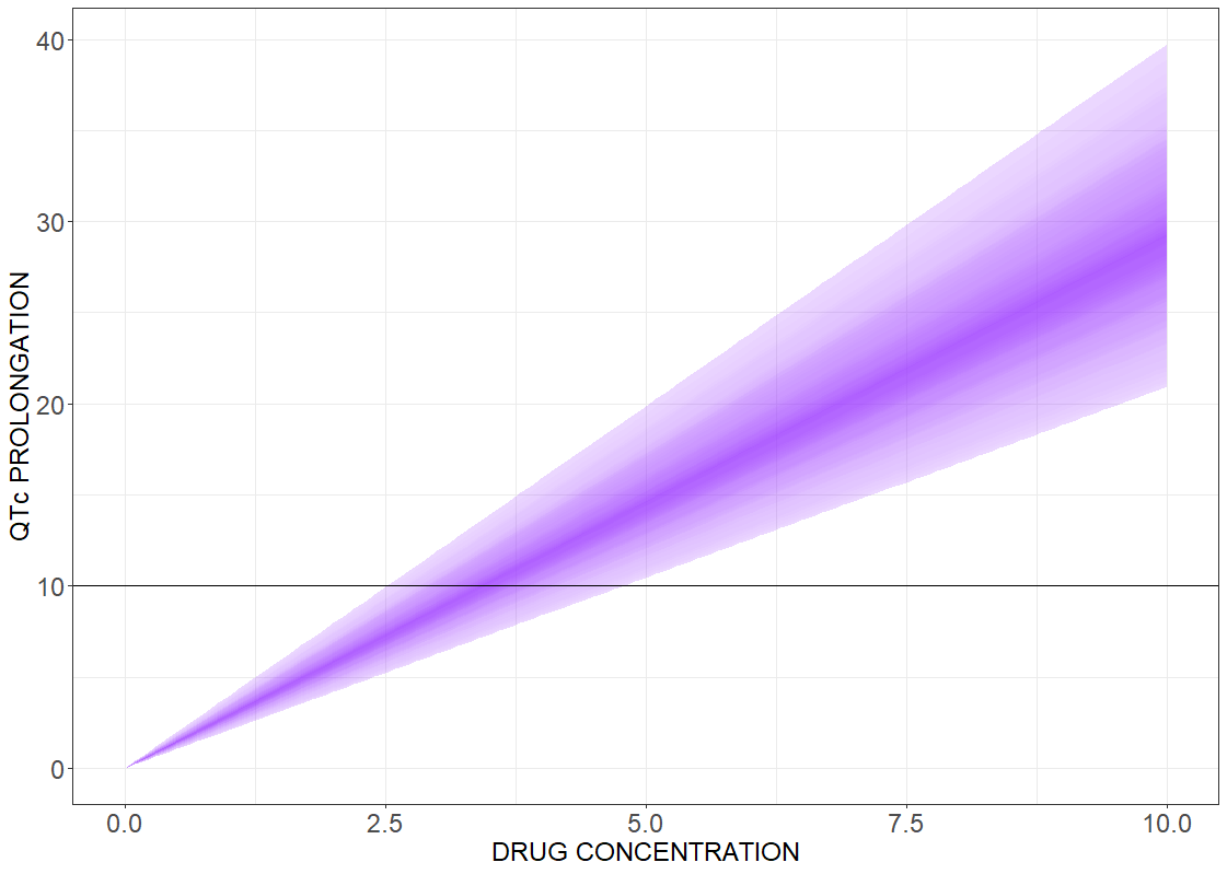
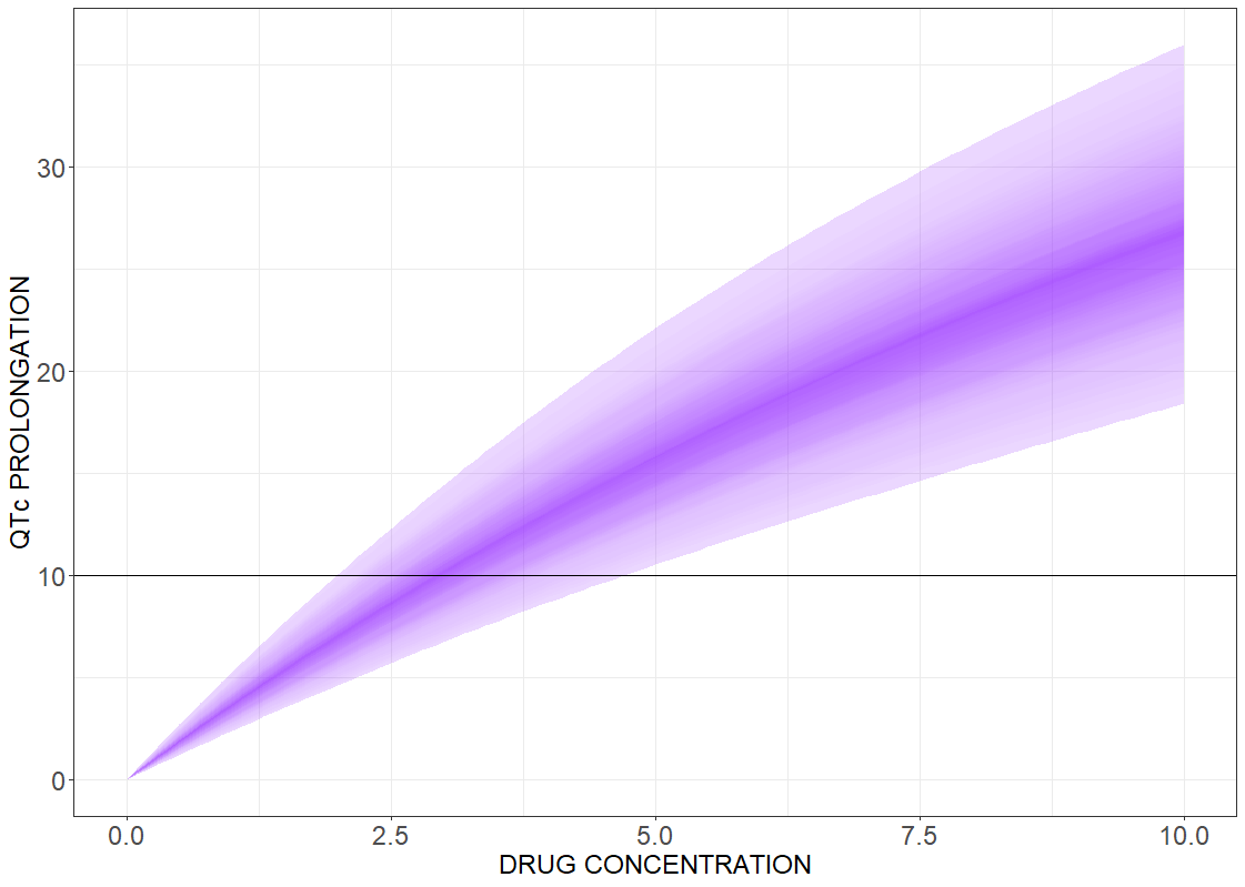
Drug induced QT interval prolongation: concentration-effect study

There is a lack of evidence for a strict correlation between a point-wise 10 ms QTc prolongation and fatal arrhythmia. Analyzing discrete results, if the maximal change in the QTc interval duration is above the 10 ms threshold value, can give false negative test results. In contrast, the concentration-effect relationship gives a continuous control of the risk as a function of drug concentration. The following figures present the results for the linear effect (on the left) and the Emax effect (on the right).

# R-script
project.file <- 'your_project_name.mlxtran'

# call the simulator
res <- simulx(project = project.file,
              group   = list(size = 200),
              output  = list("Eslope"))

# define the effect function
Cc <- seq(0,10,by=0.1)
J <- length(Cc)
S <- N*J
dfE <- data.frame(id=integer(S), conc = numeric(S), effect = numeric(S))

for (i in seq(1,N,by=1)) {
  print(i)
  for (j in seq(1,J,by=1)) {
    dfE$id[(i-1)*J + j] <- i
    dfE$conc[(i-1)*J + j] <- Cc[j]
    dfE$effect[(i-1)*J + j] <- res$parameter$Eslope[i] * Cc[j]  
  }
}

# generate plot
p <- prctilemlx(dfE, band=list(number=75, level=90)) + theme(legend.position="none") + geom_hline(yintercept=10)
                 theme(axis.text = element_text(size=18), axis.title=element_text(size=18)) + 
                 xlab('DRUG CONCENTRATION') + ylab('QTc PROLONGATION')
print(p)