Part 3: Parallel first-order absorptions

In this section we will show step-by-step how to set up a project with a model of parallel delayed two first-order absorptions.

1/ Initialization with one absorption
2/ Model with two first-order absorptions
3/ Assessing the estimate uncertainties
4/ Adjusting the residual error model
5/ Assessing over-parameterization with correlation matrix and convergence assessment
6/ Predictive power of the final model

After creating a new project in Monolix, the dataset is loaded, with the default column-types.

1/ Initialization with one absorption

To help initializing the parameter estimates, we will first estimate a model with one absorption before adding the second one.

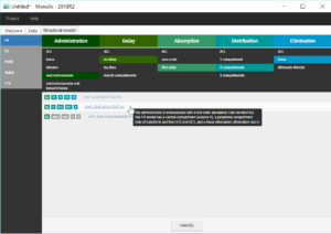
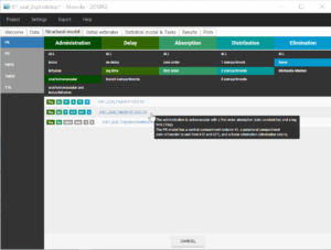
We have seen with the data exploration that a two-compartments model seems to be needed for some individuals. Therefore, we start with a model with two compartments, a first-order absorption and a linear elimination. This model is available in the PK library with two different parameterizations, under the names oral1_2cpt_kaVkk12k21.txt and oral1_2cpt_kaClV1QV2.txt, as seen below. We choose the model encoded with rates: oral1_2cpt_kaVkk12k21.txt.

After choosing the model, the tab “Initial estimates” allows to choose initial values for the five population parameters. Choosing ka_pop=5, V_pop=0.2, k_pop=0.2, k12_pop=0.1 and k21_pop=0.1 gives a rough fit for most individuals, as seen on the figure below. The log scale selected for the Y axis permits to check that two slopes are visible for the elimination, characterizing the second compartment.

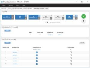
We validate these initial values by clicking on “Set as initial values”. The tab “Statistical model & Tasks” is then displayed, and can be used to adjust the statistical model as well as run some tasks to evaluate the full model.

In this first modelling phase, we aim at building in several steps the structural model, therefore we first keep the default statistical model: it is composed of a combined residual error model with an additive and a proportional term, log-normal distributions for the five parameters ka, V, k, k12 and k21 and random effects on all parameters. We also neglect for now correlations between random effects.

Once all the elements of the model have been specified, several tasks can be run in the “Statistical model & Tasks” tab to estimate the parameters and evaluate the fit to the data. It is important to save the project before (Menu > Save), so that the result text files of all tasks run afterwards will be saved in a folder next to the project file. We save the project in project_1.mlxtran.

To evaluate quickly the model, we first select in the scenario the task “Population parameters” and “EBEs” to estimate the population parameters and individual parameters. We also select the task “Conditional Distribution” which improves the performance of the diagnostic plots, in particular when there are few individuals like here. Finally, the task “Plots” is also selected to diagnose the model. We can then run this scenario by clicking on the green arrow.

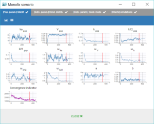
The window “Monolix scenario” allows to check in real-time the process of each task. In particular, the graphical report of SAEM iterations is useful to check that the convergence seems good.

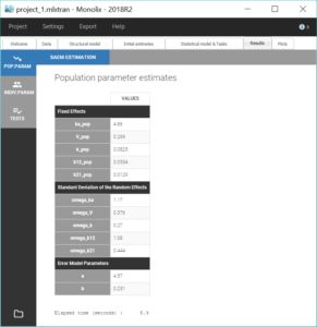
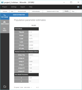
Two new tabs now display the results of the tasks. The tab “Results” contains the estimated parameters as tables, for example the population parameters shown below. Here, we can notice a high value for omega_k12, meaning a high inter-individual variability for k12, which is coherent with the variability in the shapes of eliminations that we have seen in the data viewer. We will see in a later section how to check the uncertainty of the parameters and assess the relevance of inter-individual variabilities.

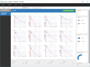
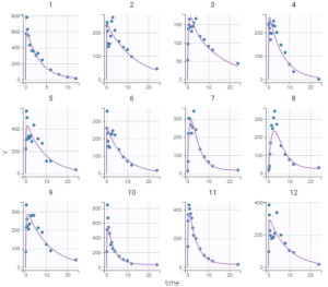
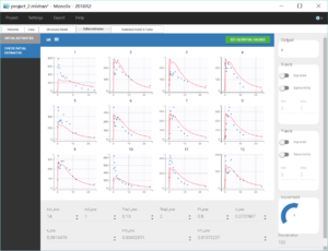
The tab “Plots” contains the diagnostic plots. Among these, the plot “Individual fits”, displayed on the figure below, allows to see that rough individual fits have been found with this first model, that do not capture the double peaks but fit properly the elimination.

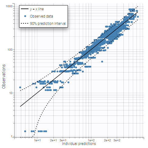
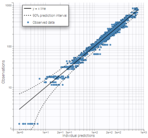
On the plot “Observations vs predictions”, displayed below on log-log scale, several over-predicted outliers can be seen outside the 90% prediction interval, suggesting a mis-specification of the structural model. The interactive plot allows to identify the corresponding individuals: hovering on a dot gives the id and time, and highights all the dots for the same individual.

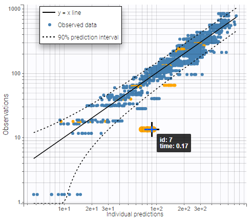
Notice that each time point corresponds to several dots, corresponding to different predictions for one observation, based on different individual parameters drawn from the conditional distribution. This method circumvents the phenomenon of shrinkage, as explained on this page.

Mots outliers correspond to low times: 0.17h for the individuals 10 and 12, 0.17h and 0.33h for the individual 7, 0.33h and 0.5h for individual 8.

Going back to the plot of the individual fits, the linked zoom on the X axis can be used to focus on low times for all individuals, as seen on the figure below. It is also possible to choose an interval to display on the X-axis in the section “Axes” of the panel “Settings”.

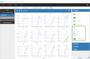
We can see that the predicted absorption starts too early for individuals 7, 8, 10 and 12, hence the over-predictions at low times. This suggests to include a delay for the oral absorption in the structural model.

Before modifying the structural model, it is possible to store the population estimates as new initial values for the next estimation, in order to speed up the convergence. This is done by clicking on “Use last estimates” in the tab “Initial estimates”. Then in the tab “Structural model”, we choose a new structural model from the library, with a delayed first-order absorption: oral1_2cpt_TlagkaVkk12k21.txt

This model has one additional parameter Tlag compared to the previous one. In the tab “Initial estimates”, we can set a reasonable initial value for Tlag_pop. According to the individual fits, this value should be between 0 and 0.17, so we can choose for example 0.1. The initial values for the five other parameters remain equal to the previous estimates.

We can then save this modified project under the name project_2.mlxtran and run the same scenario as before. Notice in the results below that the estimates for V_pop, k_pop, k12_pop and k21_pop stayed close to the previous solution, while ka_pop has increased.

The plot “Observations vs predictions”, pictured below, now shows much less outliers.

Thus, no obvious mis-specification appears other than the second absorption peak on some individual curves, that we have already seen in the data viewer. We can now include a second delayed first-order absorption in the structural model to capture this.

2/ Model with two first-order absorptions

As previously, we store the population estimates as new initial values by clicking on “Use last estimates” in the tab “Initial estimates”. Then we modify the structural model. Starting from the 2019 version, Monolix includes a library of PK models with double absorption. Therefore, we choose a model from this library in the tab “Structural model”, with the following filtering choices: type = “first order” and delay = “lag time” for the first and second absorption, with “force longer delay” = “true” for the second absorption, distribution = “2 compartments”, and elimination = “linear”. Two models are available, and we choose the one parameterized with micro constants. The model is written with PK macros and reads:

[LONGITUDINAL]
input = {ka1, ka2, F1, Tlag1, diffTlag2, V, k, k12, k21}

EQUATION:
odeType=stiff

; Parameter transformations
Tlag2 = Tlag1 + diffTlag2

PK:

;PK model definition
compartment(cmt = 1, volume = V, concentration = Cc)
absorption(cmt = 1, ka = ka1, Tlag = Tlag1, p = F1)
absorption(cmt = 1, ka = ka2, Tlag = Tlag2, p = 1-F1)
peripheral(k12, k21)
elimination(cmt = 1, k)

OUTPUT:
output = Cc
table = Tlag2

So each dose is then split into two fractions F1 and 1-F1, which are absorbed with first-order absorptions with different absorption rates and different delays. The parameter transformation for Tlag2 ensures that the second absorption starts after the first absorption. Only diffTlag2 is estimated in Monolix, however the value for Tlag2 will be available in the result folder thanks to the table statement.

The implementation with PK macros takes advantage of the analytical solution if it is available, which is the case here. Note that the syntax for each section of a Mlxtran model, such INPUT, OUTPUT or PK, is documented here.

After loading the model, initial values have to be chosen for the new parameters. Here, ka and Tlag have also been renamed into ka1 and Tlag1, so ka1_pop and Tlag1_pop are considered as new population parameters. We can set their initial values to ka1_pop=14 and Tlag1_pop=0.13, which are close to the previous estimates for ka_pop and Tlag_pop. Then, it is important to choose initial values for the new parameters that show two peaks of absorptions to guide the convergence. We thus set the initial values ka2_pop=1, Tlag2_pop=2 and F1_pop=0.8.

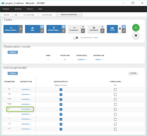
The individual parameter F1 is a fraction, so its value has to stay between 0 and 1. To make sure of this, its distribution has automatically been set to a logit-normal distribution (see figure below), because it comes from a models libray. The modified project is then saved as project_3.mlxtran.

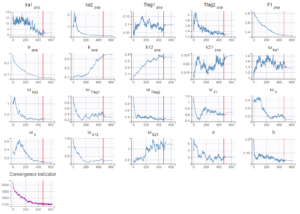
When running the same scenario as before, the convergence plot of SAEM displayed below shows that the values estimated with this model are quite different from the values estimated in the previous run, for instance the volume has decreased by half.

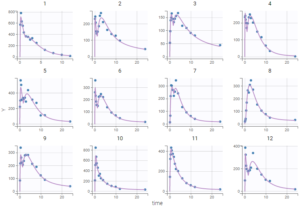
As can be seen on the plots of the individual fits, the double peaks are properly captured. On the plot Observations vs predictions, there is no visible mis-specification of the structural model. We can now focus on the statistical model.

3/ Assessing the estimate uncertainties

We can now assess the uncertainties of the population estimates by running the task “Standard errors”. For a fast assessment, we choose to select “Use linearization method”. The task then quickly computes the standard error for each estimate, displayed in the table of the population parameter estimates:

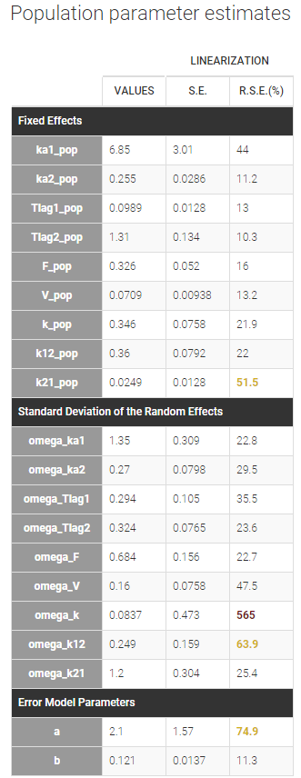
High relative standard errors are highlighted in orange or red for k21_pop, omega_k and omega_k21. They correspond to parameters that are very uncertain. In particular omega_k is difficult to identify, and its small estimated value suggests to remove the random effect on k. To confirm this hint, we are going to estimate more precisely the standard deviations of the random effects by running the estimation of the population parameters with SAEM without simulated annealing. This method may also identify other random effects that can be removed from the model.

This approach is explained in details on this page. We give here a brief summary.

By default, SAEM includes a method of simulated annealing which constrains the variance of the random effects and the residual error parameters to decrease slowly. The maximum decrease from one iteration to the next one can be set in the settings and is 5% by default.

For the first step of the modelling workflow, this option is very useful because the size of the parameter space explored by Monolix is related to the omega values. Therefore, keeping the omega values high at the beginning permits to keeps a high size for the parameter space explored by the SAEM algorithm and allows to escape local minimas to facilitate the convergence towards the global maximum.

However, once good initial values have been found and the risk of being trapped in a local maximum is negligible, the simulated annealing option may keep the omega values artificially high, even after a large number of SAEM iterations, and may prevent the identification of parameters for which the variability is in fact zero.

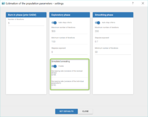
So at this point of the modelling workflow it can be useful to disable the simulated annealing, in the “Population parameters” task settings, as shown below. We do so after saving the population estimates as new initial values with “Use last estimates”.

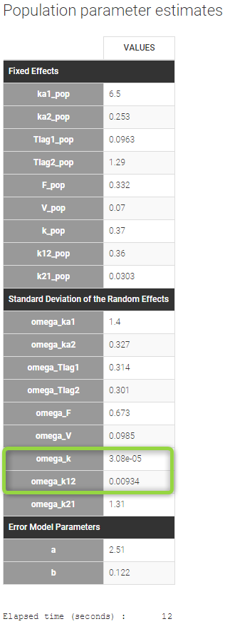
Now we save this modified project as new file project_4.mlxtran, before running SAEM. As can be seen on the table below, the estimates for omega_k and omega_k12 are now very small.

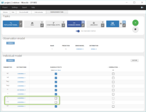
Thus, after using the last estimates, we remove the random effects for k and k12 by unchecking the corresponding boxes in the “Statistical model & Tasks tab” (as shown below), save this new project as project_5.mlxtran, and run again the tasks SAEM and Standard errors to check again the uncertainty of the estimates.

The table of the population estimates now shows reasonable standard errors. The remaining omega parameters did not decrease in spite of the disabling of the simulated annealing, therefore they were not over-estimated.

4/ Adjusting the residual error model

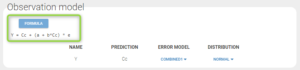
Note that the uncertainty of the constant residual error a is still quite high (74.4%). This suggests to try to find a more adequate residual error model than the “combined1” model that has been selected by default. The formula for this residual error can be seen by clicking on Formula in the Observation model:

To assess the consequences of changing the model, we first compute the log-likelihood with Importance sampling, in order to be able to check how it is affected by the modification (note that it is recommended to estimate the conditional distribution before estimating the log-likelihood):

The estimate of b is not particularly low, and is the estimate of a or b is not low either compared to the smallest observation (1.3), so neither the constant nor the proportional errors can be dropped. Therefore, after using the last estimates, we choose to try the combined2 error model, whose formula is slightly different than combined1, as shown below:

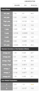
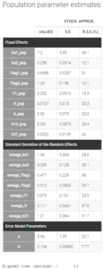
The modified project is saved as project_6.mlxtran. We run the full scenario with the task Log-likelihood. The results of the estimation of the population parameters with their standard errors is displayed below. Since this is a final assessment of the standard errors, we now choose the method Stochastic approximation rather than linearization to get precise results.

All parameter uncertainties are lower than 50%. Moreover, we can now compute again the log-likelihood and related information criteria:

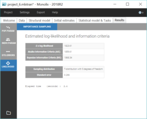
The information criteria display a significant decrease ( $\Delta$ BIC= $\Delta$ AIC=6.44), showing that the combined2 error model is more appropriate.

5/ Assessing over-parameterization with correlation matrix and convergence assessment

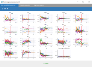
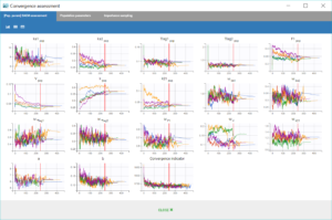
Finally, the convergence assessment tool provides a useful evaluation of the robustness of the convergence for each estimate. We choose to estimate the parameters as well as the standard errors and the log-likelihood five times, with different seeds and initial values randomly drawn around the estimate for each parameter. The graphical report is show below. The panel on the left allows to compare the convergences across the five runs, while the panel on the right compares the resulting estimates along with confidence intervals based on their standard errors.

We notice that the convergence is robust with close results between runs for most parameters. However, the estimates of k_pop and k21_pop show significant variability, with two possible sets of estimates found for each parameter. This is characteristics of correlated estimates, and this can be confirmed by looking at the correlation matrix of the estimates, in the results of the task “Standard errors”, as displayed in the following figure.

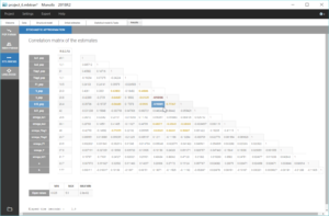
The correlations between V_pop and k_pop is quite high, as well as between V_pop and k12_pop. This means that k and k12 have opposite effects to V on the prediction, and the data is not rich enough to be able to identify them uniquely. The model is a bit over-parameterized, likely due to the low number of individuals. Therefore, it is necessary to fix one of these three parameters to get a robust convergence.

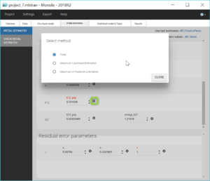
We choose to fix k12_pop in the final model saved in project_7.mlxtran, to keep the inter-individual variability in elimination. This is done in the tab “Initial estimates”, by clicking on the small gear icon next to k12_pop and choosing “Fixed” for the estimation method. k12_pop appears then colored in orange.

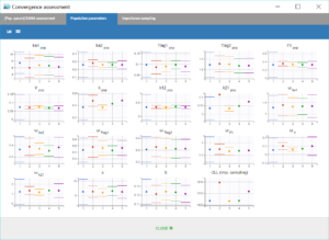
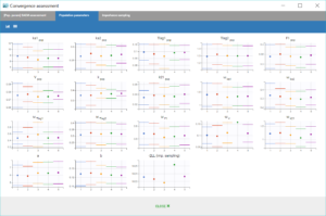
Performing again a convergence assessment on this project gives the following reports, with a reasonably robust convergence of each estimate.

6/ Predictive power of the final model

The final model has been selected after a step-by-step workflow alternating an evaluation of the model and adjustment of one element.

The predictive power of the final model can now be assessed by generating the VPC, shown below.

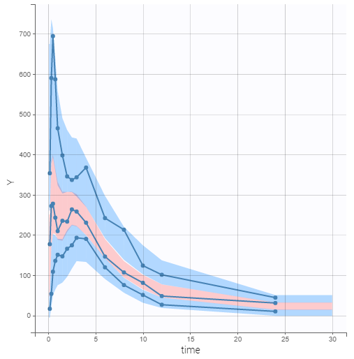
On this figure, the empirical median and percentiles displayed as blue curves show good agreement with the predicted median and percentiles displayed as pink and blue areas respectively. Simulations of the model are thus able to predict both the central trend, that exhibit a double peak, and variability of the dataset.

In conclusion, we have been able to build a model step-by-step in Monolix, that captures well the double peaks in the PK of veralipride. The final model had one fixed parameter, characterizing a slight over-parameterization, and showed a good predictive power.

Continue to Part 4: Model of double absorption site

Case study: Model of double absorption of veralipride – Part 3