- Part 1: Introduction
- Part 2: Data exploration with Datxplore
- Part 3: Parallel first-order absorptions
- Part 4: Model of double absorption site
- Part 5: Simulations
Part 4: Model of double absorption site
In this section, we will apply and evaluate a model from the literature.
- 1/ Model writing with macros and ODEs
- 2/ Model exploration with Mlxplore
- 3/ Model estimation and diagnosis with Monolix
This model has been published in:
Godfrey, KR, Arundel, PA, Dong, Z, Bryant, R (2011). Modelling the Double Peak Phenomenon in pharmacokinetics. Comput Methods Programs Biomed, 104, 2:62-9.
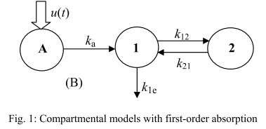
It is based on an approach that strives to ensure a clear physiological interpretation. Site-specific absorption has been suggested to be the major mechanism responsible for the multiple peaking phenomenon for veralipride, with rapid absorption occurring in the proximal part of the gastrointestinal tract, followed by a second absorption phase in more distal regions. Thus, the model describes two absorption sites with discontinuous input rate of the drug, as represented below (figures from (Godfrey et al., 2011)).
 |
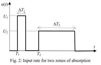 |
The absorption is done in two successive sites defined as two time windows during which a constant input rate of the drug is applied. Moreover, an identical absorption rate is assumed for the two absorption windows. Defining precisely each time phase brings some complexity in the model, which requires in total 10 parameters.
We present two implementations of this model, one with ODEs and one with PK macros.
1/ Model writing with macros and ODEs
It is possible to write the structural model with PK macros by modelling the constant input rate as two zero-order absorptions of the drug in a compartment representing the gut. The drug amount is split between these two absorptions with a parameter F1 representing the fraction of the drug absorbed at the first site. A transfer macro then encodes the identical absorption from each absorption site to the central compartment.
The model file is displayed below. Note that the model is very easy to read with only seven macros. Detailed documentation pages are available for the macros compartment, elimination, peripheral, absorption, transfer.
[LONGITUDINAL]
input={V, ka, k, k12, k21, T1, dT1, T2, dT2, F1}

EQUATION:
odeType=stiff

PK:
; Define central and peripheral compartment
compartment(cmt=1, volume=V, concentration=Cc)
elimination(cmt=1, k)
peripheral(k12,k21)

; Define gut compartment with two zero-order inputs
compartment(cmt=3, amount=Ag)
absorption(cmt=3,Tlag=T1, Tk0=dT1, p=F1)
absorption(cmt=3, Tlag=T1+dT1+T2, Tk0=dT2, p=1-F1)

; Absorption of drug from gut compartment
transfer(from=3,to=1,kt=ka)

OUTPUT:
output={Cc}
Several remarks:
-While in the publication the parameter T2 represents the time at which the second absorption starts, here it represents the time between the end of the first absorption and the start of the second absorption. This parameterization ensures that there is no time overlap between each absorption site.
-The transfer rates U1 and U2 from the publication do not appear explicitly. Zero-order absorptions defined with the macro absorption are equivalently defined with the duration of the transfer and the fraction of the dose used during each transfer. Nonetheless, the transfer rates can be retrieved with the equations: U1=amtDose*F1/dT1 and U2=amtDose*(1-F1)/dT2, where amtDose is the drug amount administered.
-PK macros have the advantage of taking into account analytical solutions when they are available. Here, because of the transfer between the gut and the central compartment, no analytical solution is available. Thus the model has to be simulated by integration. The statement odeType=stiff is therefore important to choose a stable integration solver.
The same model can also be written with ODEs as shown below. The model counts four ODEs for Ad, Ag, Ac and Ap, which represent respectively the drug amount in the depot compartment, the gut, the central compartment and the peripheral compartment. The ODEs are linked to the drug administration information with amtDose, which is a keyword recognized by Mlxtran as the drug amount administered (see all dose-related keywords). A zero-order transfer is implemented between Ad and Ag, the drug amount in the gut. A time-dependence is encoded for the transfer rate with if/else statements. Note that because the zero-order transfer is independent from system variables, the variable Ad is actually optional in this model. However, it is interesting to keep it to visualize the drug consumption.
[LONGITUDINAL]
input={V, ka, k, k12, k21, T1, dT1, T2, dT2, F1}

EQUATION:
odeType=stiff

t_0 = 0
Ag_0 = 0
Ac_0 = 0
Ap_0 = 0
Ad_0 =amtDose

U1=amtDose*F1/dT1
U2=amtDose*(1-F1)/dT2

if t<=T1
  u=0
elseif t<=T1+dT1
  u=U1
elseif t<=T1+dT1+T2
  u=0
elseif t<=T1+dT1+T2+dT2
  u=U2
else
  u=0
end

ddt_Ad = -u
ddt_Ag = -ka*Ag+u
ddt_Ac = ka*Ag-(k+k12)*Ac+k21*Ap
ddt_Ap = k12*Ac-k21*Ap

Cc=Ac/V

OUTPUT:
output={Cc}
2/ Model exploration with Mlxplore
Mlxplore is an application dedicated to visual exploration of a model behaviour, with easy assessment of the parameters influence.
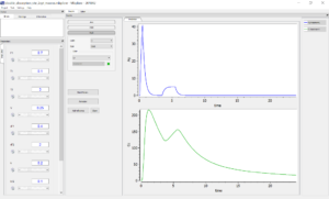
It is then useful here to check that the two models are equivalent with the same simulation results. The ability to display any variable of the model also provides insightful simulations to understand how the model behaves. Below we show the results of simulations of each model with Mlxplore, with the same parameter values.
For the first model written with macros, it is possible to output the amount of drug in the gut and the concentration in the central compartment. However, the depot compartment is defined implicitly and its value is not available.
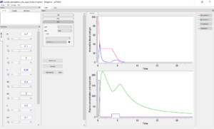
In contrast, in the second model the amounts of drug in each compartment had to be explicitly defined, and it is possible to plot them as outputs, as well as the input rate. This permits a graphical visualization of each system variable over time: on the figure below, the drug amount in the depot compartment and the gut compartments are displayed on the top, and the plasma concentration is overlaid with the input rate on the bottom.
3/ Model estimation and diagnosis with Monolix
Since we have verified that both models are equivalent, we can choose any of them to use in Monolix. Similarly to the Part 3 of this case study, we can apply a step-by-step modelling workflow with the following steps, using at each step the last estimates as new initial values for the next run:
–project_1.mlxtran: a preliminary fit is made with a single absorption zone only. We can set all parameters for the second site to zero, or fix F1=1 with no inter-individual variability. The parameters T2 and dT2 can be fixed as well to speed-up the estimation. Appropriate initial estimates have to be chosen for the fixed effects. Here we took T1_pop=0.1, V_pop=0.22, dT1_pop=1, k12_pop=k21_pop=0.1, k_pop=0.2, ka_pop=2.
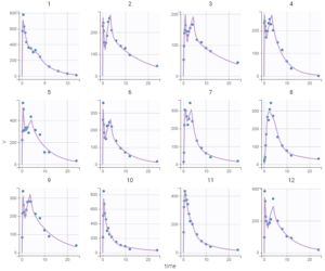
–project_2.mlxtran: in the second project all parameters are then unfixed, a logit-normal distribution is chosen for F1 and a new estimation with SAEM is performed. The individual fits show that the model is able to capture the double peaks. In contrast with the model from the Part 3 of this case study, the finite absorption sites allow to predict pointed peaks.
–project_3.mlxtran: since the estimates should now be close to the global solution, the simulated annealing option can be disabled in the settings of SAEM. After running again, the estimate for omega_dT2 becomes close to zero (1e-5), we can then remove the random effect for dT2 in the next project.
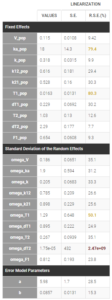
–project_4.mlxtran: After running again, the correlation matrix of the estimates computed with linearization shows a large correlation between k_pop and V_pop. The model is over-parameterized, k_pop is then fixed in the next project.
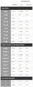
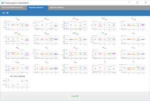
– project_5.mlxtran: We consider this as the final model. Although there are still some quite high uncertainties on population parameters, a convergence assessment shows a reasonable robustness.
 |
 |
The VPC also shows a quite good predictive power, although there remain a few outlier areas on the second absorption peak and the end of the elimination.
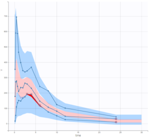
Therefore, we consider that the performance of the model built in the previous section of this case study is higher.