Part 5: Simulations

In this section we choose the model of parallel first-order absorption estimated in Part 3 to perform new simulations in Simulx. The goal is to assess the effect of the drug in different ways in a large population.

Simulx is the application of the MonolixSuite dedicated to advanced simulations. It is implemented as an R package called mlxR, which provides more flexibility than Mlxplore. Simulx can simulate a new model, or it can reuse automatically all the elements of a Monolix project for the simulation: the model, the parameters estimated in the project, as well as the design from the dataset. It is also possible to redefine manually any of these elements.

Here we are going to simulate the model based on the Monolix project built in Part 3, and we will only modify the number of individuals and the outputs, in order to output the AUC as well as the duration spent in a therapeutic window.

Simulating the model for double absorption of veralipride with AUC

We begin by opening R (for example in Rstudio) and loading the mlxR library which contains the function simulx with:

library(mlxR)

Before simulating the project, we define with the following line a formula for the AUC to add in the model, with the integration of Cc.

add <- list(formula=c("ddt_AUC = Cc"))

Then we define two outputs for the simulation: the plasma concentration Cc at different time point between 0 and 25, and the AUC only at the last time point 25.

outCc <- list(name= c("Cc"), time=seq(0,25, by=0.5))
outAUC <- list(name= c("AUC"), time=25)

These elements are then given as arguments to simulx, with the project path and the number of individuals to simulate. We choose 500 to simulate a large population.

res1 <- simulx(project = "project_7_double_first_order_oral.mlxtran",
               addlines = add,
               output = list(outCc, outAUC),
               group = list(size=500))

Note that the working directory has to be set to the folder containing the Monolix project.

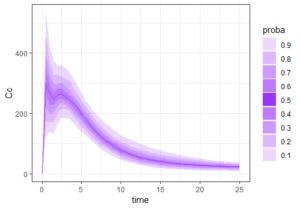
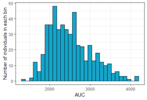
The result of the simulation is stored in the list res1, as tables named res1$Cc and res1$AUC. Because there are many individuals, the function prctilmlx of the mlxR package can be used to vizualise the predicted concentrations as percentiles. The AUC values are also saved in a table AUC in the list res1. Visualize its content as a histogram shows a large variability in the AUC values.

# Plot concentrations
prct <- prctilemlx(res1$Cc)
print(prct)

# Plot AUC
histAUC <- ggplotmlx(res1$AUC, aes(AUC))+geom_histogram(bins=30, fill='#16a4ca', color="black")+
            xlab('AUC')+ylab('Number of individuals in each bin')
print(histAUC)

Let’s investigate the shape of the concentration curves with respect to the AUC values.

We first compute the AUC quartiles, and add a column in the tables res1$AUC and res1$Cc that assigns each individual to its corresponding AUC quartile. The percentiles of the concentrations can then be plotted for each quartile.

# Compute AUC quartiles
AUCq <- quantile(res1$AUC$AUC)
names(AUCq) <- paste0("Q",0:4)

# Create column AUCq with AUC quartile of each id
res1$AUC$AUCq <- sapply(res1$AUC$AUC, function(x){names(AUCq[x<AUCq])[1]})
res1$Cc$AUCq <- factor(res1$AUC$AUCq[res1$Cc$id], levels=names(AUCq))

# Plot concentration percentiles over time, grouped by AUC quartiles
prctq <- prctilemlx(res1$Cc, group="AUCq")+ theme(legend.position = "none")
print(prctq)

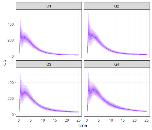
This plot shows that the subpopulation corresponding to the 4^th AUC quartile shows clear double peaks, while the second peaks corresponding to the 1^st quartile are smaller. The double peak phenomenon with a high double peak seems to increase the AUC value.

Computing a therapeutic window

We are now going to compute a therapeutic window. To this end, we add several lines in the model, that define a new variable TimeAboveTarget which is an integration of the time when each individual concentration is above a target concentration of 200. At the end of the simulation this variable will contain for each individual the duration spent above the target over the whole simulation. We define only one high measurement time in the output for this variable and we simulate the model with this variable with simulx.

# a target concentration Ctarget=200
add <- list(formula=c("Ctarget=200",
                      "TimeAboveTarget_0 = 0",
                      "if Cc > Ctarget",
                      "xTime = 1",
                      "else",
                      "xTime = 0",
                      "end",
                      "ddt_TimeAboveTarget = xTime"))

# output time for TimeAboveTarget
out <- list(name= c("TimeAboveTarget"), time=100)

# Simulation
res2 <- simulx(project = project.file,
               addlines = add,
               output = out,
               group = list(size=500))

As before, we can first visualize the result as a histogram, to see the variability in the population.

# Plot histogram of times

histTimeAboveTarget <- ggplotmlx(res2$TimeAboveTarget, aes(TimeAboveTarget))+
                        geom_histogram(bins=20, fill='#16a4ca', color="black")+
                        xlab('Time above target concentration')+
                        ylab('Number of individuals in each bin')
print(histTimeAboveTarget)

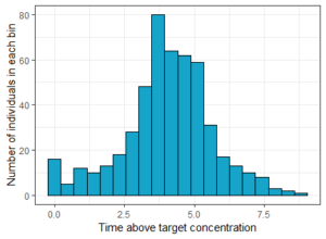
The result can then be quantified with some simple post-processing in R. In this case we compute the percentage of individuals that had a concentration above the target during at least 2h:

percentTargetTime <- sum(res2$TimeAboveTarget$TimeAboveTarget>2)/nrow(res2$TimeAboveTarget)

print(paste0("Percentage of individuals for which the concentration stays above the target during at least 2h: ",
              percentTargetTime*100,"%"))

[1] "Percentage of individuals for which the concentration stay above the target during at least 2h: 89.2%"

Conclusion

Two modelling approaches were explored and compared in this case study.

In the first approach, a model was built in Monolix with a step-by-step workflow alternating an evaluation of the model and adjustment of one element. The inter-individual variability was precisely assessed to identify non-varying parameters. Due to the small size of the dataset, over-parameterization should be a concern, and was identified with the correlation matrix of the estimates and convergence assessment. The final model has one fixed parameter, characterizing a slight over-parameterization, and shows a good predictive power.

In the second approach, a model with two successive absorption windows was chosen to reflect a physiological interpretation. The model was first written with PK macros, which facilitate model writing and reading, and the behavior of the model was explored with Mlxplore. An equivalent implementation with ODEs was also written to take advantage of the availability of each system variable in Mlxplore. Finally, the model was estimated and diagnosed in Monolix. Interestingly, it provided quite different individual predictions, since the finite absorption sites allow to predict pointed peaks with higher absorption rates. However, the predictive power assessed by the VPC was not as good as in the first case.

Finally, the first model was selected for simulations, and we have used Simulx to obtain easily new useful outputs to assess the effect of the drug in a large population.

Case study: Model of double absorption of veralipride – Part 5

Part 5: Simulations

Simulating the model for double absorption of veralipride with AUC

Computing a therapeutic window

Conclusion