- Introduction
- Defining the residual error model from the Monolix GUI
- Some basic residual error models
- Residual error models for bounded data
- Autocorrelated residuals
- Using different error models per group/study
Objectives: learn how to use the predefined residual error models.
Projects: warfarinPK_project, bandModel_project, autocorrelation_project, errorGroup_project
Introduction
For continuous data, we are going to consider scalar outcomes (\(y_{ij} \in \mathbb{R}\)) and assume the following general model:
$$y_{ij}=f(t_{ij},\psi_i)+ g(t_{ij},\psi_i,\xi)\varepsilon_{ij}$$
for i from 1 to N, and j from 1 to \(\text{n}_{i}\), where \(\psi_i\) is the parameter vector of the structural model f for individual i. The residual error model is defined by the function g which depends on some additional vector of parameters \(\xi\). The residual errors \((\varepsilon_{ij})\) are standardized Gaussian random variables (mean 0 and standard deviation 1). In this case, it is clear that \(f(t_{ij}, \psi_i)\) and \(g(t_{ij}, \psi_i, \xi)\) are the conditional mean and standard deviation of \(y_{ij}\), i.e.,
$$\mathbb{E}(y_{ij} | \psi_i) = f(t_{ij}, \psi_i)~~\textrm{and}~~\textrm{sd}(y_{ij} | \psi_i)= g(t_{ij}, \psi_i, \xi)$$
Available error models
In Monolix, we only consider the function g to be a function of the structural model f, i.e. \(g(t_{ij}, \psi_i, \xi)= g(f(t_{ij}, \psi_i), \xi)\) leading to an expression of the observation model of the form
$$y_{ij}=f(t_{ij},\psi_i)+ g(f(t_{ij}, \psi_i), \xi)\varepsilon_{ij}$$
The following error models are available:
- constant : \(y = f + a \varepsilon\). The function g is constant, and the additional parameter is \(\xi=a\)
- proportional : \(y = f + bf^c \varepsilon\). The function g is proportional to the structural model f, and the additional parameters are \(\xi = (b,c)\). By default, the parameter c is fixed at 1 and the additional parameter is
.
- combined1 : \(y = f + (a+ bf^c) \varepsilon\). The function g is a linear combination of a constant term and a term proportional to the structural model f, and the additional parameters are \(\xi = (a, b)\) (by default, the parameter c is fixed at 1).
- combined2 : \(y = f + \sqrt{a^2+ b^2(f^c)^2} \varepsilon\). The function g is a combination of a constant term and a term proportional to the structural model f (g = bf^c), and the additional parameters are \(\xi = (a, b)\) (by default, the parameter c is fixed at 1).
 .
.Notice that the parameter c is fixed to 1 by default. However, it can be unfixed and estimated.
The assumption that the distribution of any observation \(y_{ij}\) is symmetrical around its predicted value is a very strong one. If this assumption does not hold, we may want to transform the data to make it more symmetric around its (transformed) predicted value. In other cases, constraints on the values that observations can take may also lead us to transform the data.
Available transformations
The model can be extended to include a transformation of the data:
$$u(y_{ij})=u(f(t_{ij},\psi_i)) + g(u(f(t_{ij},\psi_i)) ,\xi) $$
As we can see, both the data \(y_{ij}\) and the structural model f are transformed by the function u so that \(f(t_{ij}, \psi_i)\) remains the prediction of \(y_{ij}\). Classical distributions are proposed as transformation:
- normal: u(y) = y. This is equivalent to no transformation.
- lognormal: u(y) = log(y). Thus, for a combined error model for example, the corresponding observation model writes \(\log(y) = \log(f) + (a + b\log(f)) \varepsilon\). It assumes that all observations are strictly positive. Otherwise, an error message is thrown. In case of censored data with a limit, the limit has to be strictly positive too.
- logitnormal: u(y) = log(y/(1-y)). Thus, for a combined error model for example, the corresponding observation model writes \(\log(y/(1-y)) = \log(f/(1-f)) + (a + b\log(f/(1-f)))\varepsilon\). It assumes that all observations are strictly between 0 and 1. It is also possible to modify these bounds and not “impose” them to be 0 and 1, i.e. to define the logit function between a minimum and a maximum: the function u becomes u(y) = log((y-y_min)/(y_max-y)). Again, in case of censored data with a limit, the limits too must belong strictly to the defined interval.
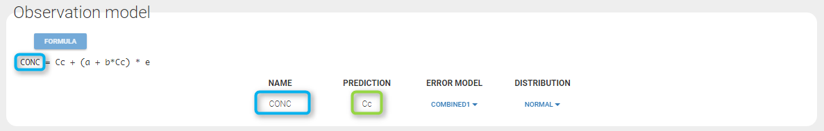
Any interrogation on what is the formula behind your observation model? There is a button FORMULA on the interface as on the figure below where the observation model is described linking the observation (named CONC in that case) and the prediction (named Cc in that case). Note that \(\epsilon\) is noted e here.
Remarks: In previous Monolix version, only the error was available. Thus, what happens to the errors that are not proposed anymore? Is it possible to have “exponential”, “logit”, “band(0,10)”, and “band(0,100)”? Yes, in this version, we choose to split the observation model between its error model and its distribution. The purpose is to have a more unified vision of models and increase the number of possibilities. Thus, here is how to configure new projects with the previous error model definition.
- “exponential” is an observation model with a constant error model and a lognormal distribution.
- “logit” is an observation model with a constant error model and a logitnormal distribution.
- “band(0,10)” is an observation model with a constant error model and a logitnormal distribution with min and max at 0 and 10 respectively.
- “band(0,100)” is an observation model with a constant error model and a logitnormal distribution with min and max at 0 and 100 respectively.
Defining the residual error model from the Monolix GUI
A menu in the frame Statistical model|Tasks of the main GUI allows one to select both the error model and the distribution as on the following figure (in green and blue respectively)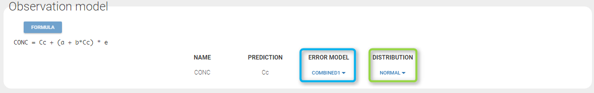
A summary of the statistical model which includes the residual error model can be displayed by clicking on the button formula.
Some basic residual error models
- warfarinPKlibrary_project (data = ‘warfarin_data.txt’, model = ‘lib:oral1_1cpt_TlagkaVCl.txt’)
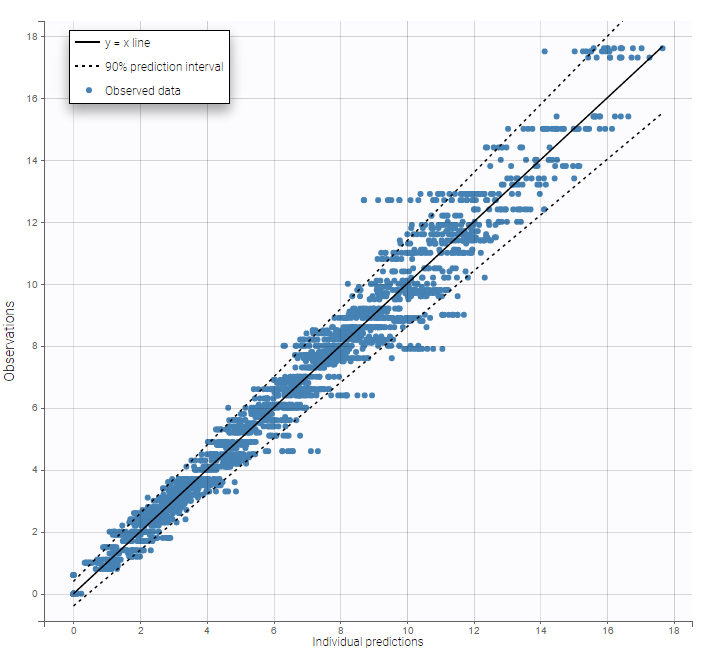
The residual error model used with this project for fitting the PK of warfarin is a combined error model, i.e. \(y_{ij} = f(t_{ij}, \psi_i))+ (a+bf(t_{ij}, \psi_i)))\varepsilon_{ij}\) Several diagnosis plots can then be used for evaluating the error model. The observation versus prediction figure below seems ok.
Remarks:
- Figures showing the shape of the prediction interval for each observation model available in Monolix are displayed here.
- When the residual error model is defined in the GUI, a bloc DEFINITION: is then automatically added to the project file in the section [LONGITUDINAL] of <MODEL> when the project is saved:
DEFINITION:
y1 = {distribution=normal, prediction=Cc, errorModel=combined1(a,b)}
Residual error models for bounded data
- bandModel_project (data = ‘bandModel_data.txt’, model = ‘lib:immed_Emax_null.txt’)
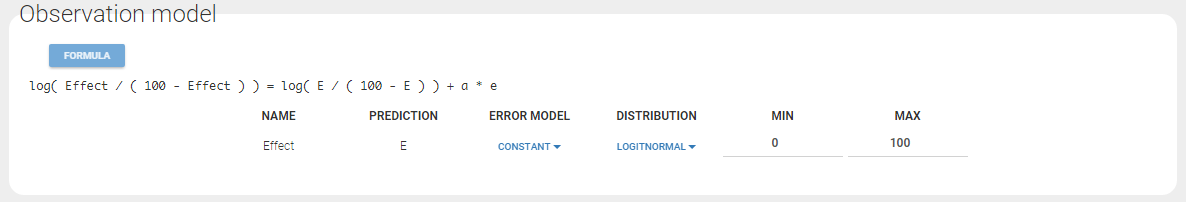
In this example, data are known to take their values between 0 and 100. We can use a constant error model and a logitnormal for the transformation with bounds (0,100) if we want to take this constraint into account.
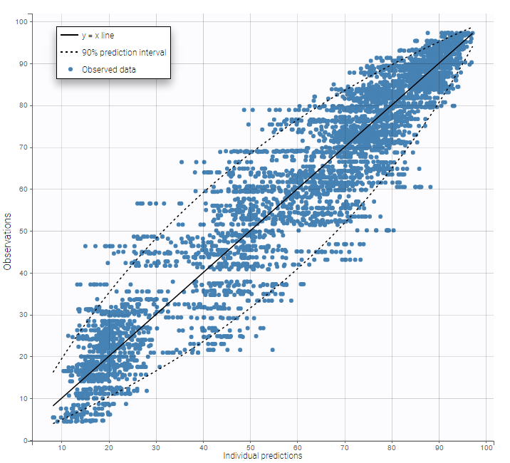
In the Observation versus prediction plot, one can see that the error is smaller when the observations are close to 0 and 100 which is normal. To see the relevance of the predictions, one can look at the 90% prediction interval. Using a logitnormal distribution, we have a very different shape of this prediction interval to take that specificity into account.
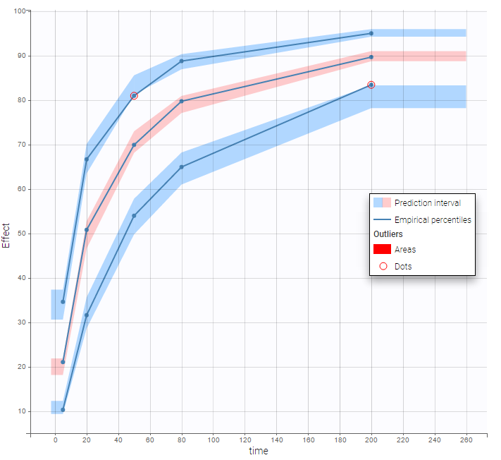
VPCs obtained with this error model do not show any mispecification
 This residual error model is implemented in
 Mlxtran as follows:
DEFINITION:
effect = {distribution=logitnormal, min=0, max=100, prediction=E, errorModel=constant(a)}
Autocorrelated residuals
For any subject i, the residual errors \((\varepsilon_{ij},1 \leq j \leq n_i)\) are usually assumed to be independent random variables. The extension to autocorrelated errors is possible by assuming, that \((\varepsilon_{ij})\) is a stationary autoregressive process of order 1, AR(1), which autocorrelation decreases exponentially:
$$ \textrm{corr}(\varepsilon_{ij},\varepsilon_{i,{j+1}}) = r_i^{(t_{i,j+1}-t_{ij})}$$
where \(0 \leq r_i \leq 1\) for each individual i. If \(t_{ij}=j\) for any (i,j), then \(t_{i,j+1}-t_{i,j}=1\) and the autocorrelation function \(\gamma_i\)for individual i is given by
$$\gamma_i(\tau) = \textrm{corr}(\varepsilon_{ij}, \varepsilon_{i,j+\tau}) = r_i^{\tau}$$
The residual errors are uncorrelated when \(r_i=0\).
- autocorrelation_project (data = ‘autocorrelation_data.txt’, model = ‘lib:infusion_1cpt_Vk.txt’)
Autocorrelation is estimated since the checkbox r is ticked in this project: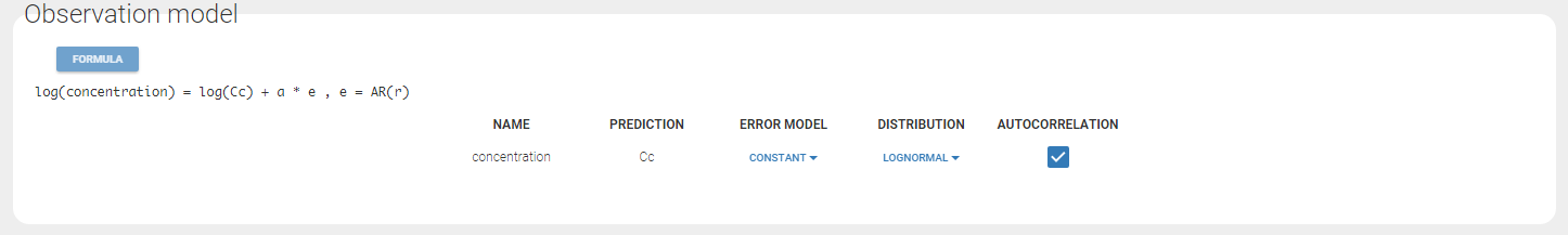 Estimated population parameters now include the autocorrelation r:
 Important remarks:
Monolixaccepts both regular and irregular time grids.- For a proper estimationg of the autocorrelation structure of the residual errors, rich data is required (i.e. a large number of time points per individual) .
- To add autocorrelation, the user should either use the connectors, or write it directly in the Mlxtran
- add “autoCorrCoef=r” in definition “DV = {distribution=normal, prediction=Cc, errorModel=proportional(b), autoCorrCoef=r}” for example
- add “r” as an input parameter.
Using different error models per group/study
- errorGroup_project (data = ‘errorGroup_data.txt’, model = ‘errorGroup_model.txt’)
Data comes from 3 different studies in this example. We want to have the same structural model but use different error models for the 3 studies. A solution consists in defining the column STUDY with the reserved keyword OBSERVATION ID. It will then be possible to define one error model per outcome: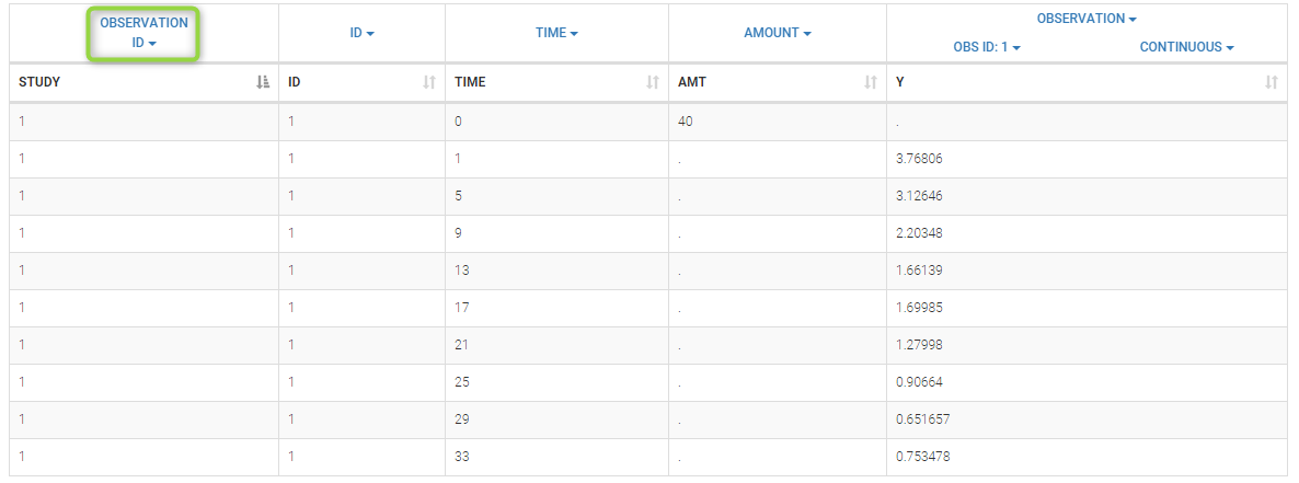
Here, we use the same PK model for the 3 studies:
[LONGITUDINAL]
input = {V, k}

PK:
Cc1 = pkmodel(V, k)
Cc2 = Cc1
Cc3 = Cc1

OUTPUT:
output = {Cc1, Cc2, Cc3}
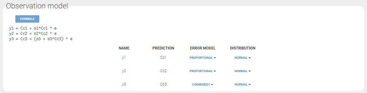
Since 3 outputs are defined in the structural model, one can now define 3 error models in the GUI:
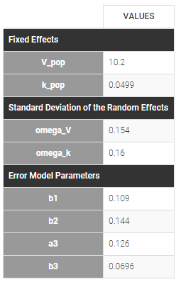
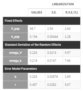
 Different residual error parameters are estimated for the 3 studies. One can remark than, even if 2 proportional error models are used for the 2 first studies, different parameters b1 and b2 are estimated: