- Introduction
- Occasion definition in a data set
- Cross over study
- Occasions with washout
- Occasions without washout
- Multiple levels of occasions
Objectives: learn how to take into account inter occasion variability (IOV).
Projects: iov1_project, iov1_Evid_project, iov2_project, iov3_project, iov4_project
Introduction
A simple model consists of splitting the study into K time periods or occasions and assuming that individual parameters can vary from occasion to occasion but remain constant within occasions. Then, we can try to explain part of the intra-individual variability of the individual parameters by piecewise-constant covariates, i.e., occasion-dependent or occasion-varying (varying from occasion to occasion and constant within an occasion) ones. The remaining part must then be described by random effects. We will need some additional notation to describe this new statistical model. Let
- \(\psi_{ik}\) be the vector of individual parameters of individual i for occasion k, where \(1\leq i \leq N\) and \(1\leq k \leq K\).
- \({c}_{ik}\) be the vector of covariates of individual i for occasion k. Some of these covariates remain constant (gender, group treatment, ethnicity, etc.) and others can vary (weight, treatment, etc.).
Let \(\psi_i = (\psi_{i1}, \psi_{i2}, \ldots , \psi_{iK})\) be the sequence of K individual parameters for individual i. We also need to define:
- \(\eta_i^{(0)}\), the vector of random effects which describes the random inter-individual variability of the individual parameters,
- \(\eta_{ik}^{(1)}\), the vector of random effects which describes the random intra-individual variability of the individual parameters in occasion k, for each \(1\leq k \leq K\).
Here and in the following, the superscript (0) is used to represent inter-individual variability, i.e., variability at the individual level, while superscript (1) represents inter-occasion variability, i.e., variability at the occasion level for each individual. The model now combines these two sequences of random effects:
\(h(\psi_{ik}) = h(\psi_{\rm pop})+ \beta(c_{ik} – c_{\rm pop}) + \eta_i^{(0)} + \eta_{ik}^{(1)} \)
Remark: Individuals do not need to share the same sequence of occasions: the number of occasions and the times defining the occasions can differ from one individual to another.
Occasion definition in a data set
There are two ways to define occasions in a data set:
- Explicitly using an OCCASION column. It is possible to have, in a data set, one or several columns with the column-type OCCASION. It corresponds to the same subject (ID should remain the same) but under different circumstances, occasions. For example, if the same subject has two successive different treatments, it should be considered as the same subject with two occasions. The OCC columns can contain only integers.
- Implicitly using EVID column. If there is an EVID column with a value 4 then Monolix defines a washout and creates an occasion. Thus, if there are several times where EVID equals 4 for a subject, it will create the same number of occasions. Notice that if EVID equals 4 happens only once at the beginning, only one occasion will be defined and no inter occasion variability would be possible.
There are three kinds of occasions
- Cross over study: In that case, data is collected for each patient during two independent treatment periods of time, there is an overlap on the time definition of the periods. A column OCCASION can be used to identify the period. An alternative way is to define an EVID column starting for all occasions with EVID equals 4. Both types of definition will be presented in the iov1 example.
- Occasions with washout: In that case, data is collected for each patient during one period and there is no overlap between the periods. The time is increasing but the dynamical system (i.e. the compartments) is reset when the second period starts. In particular, EVID=4 indicates that the system is reset (washout) for example, when a new dose is administrated.
- Occasions without washout: In that case, data is collected for each patient during one period and there is no overlap between the periods. The time is increasing and we want to differentiate periods in terms of occasions without any reset of the dynamical system. Multiple doses are administrated to each patient. each period of time between successive doses is defined as a statistical occasion. A column OCCASION is therefore necessary in the data file to define it.
Cross over study
- iov1_project (data = ‘iov1_data.txt’, model = ‘lib:oral1_1cpt_kaVk.txt’)
In this example, PK data is collected for each patient during two independent treatment periods of time (each one starting at time 0). A column OCCASION is used to identify the study:
This column is defined using the reserved keyword OCCASION. Then, the model associated to the individual parameter is as presented below
 First, to define the variability of each parameter on each level, you just have to go on the good level, and you’ll see the associated random effects on each level. On the figure above, we see that all parameters have variability on the ID level, which means that all parameters have inter-individual variability. On the figure below, we see the OCC level. In the presented case, only the volume V has inter-study variability and thus inter occasion variability. Thus, this is the only one having variability on the occasion level.
In terms of covariates, we then see two parts as displayed below. We see the covariates
- associated to the level ID (in green). It corresponds to all the covariates that are constant for each subject.
- associated to the level OCC (in blue). It corresponds to all the covariates that are constant for each occasion but not on each subject.
In the presented case, the treatment TRT varies for each individual. It contains inter-occasion information and is thus displayed with the occasion level. On the other hand, the SEX is constant for each subject. It contains then inter-individual information but no inter-occasion information. It is then displayed with the ID level.
 What is the impact?
Covariates can be associated to the parameter if and only if their level of variability is coherent with the level of variability of the parameter. In the presented case,
- TRT has inter-occasion variability. It can only be used with the parameter V that has inter-occasion variability. The two other parameters have only inter-individual variability and can therefore not use this TRT information. The interface is greyed and the user can not add this covariate to the parameters ka and Cl.
- SEX has only inter-individual variability. It can therefore be associated to any parameter that has inter-individual variability.
The population parameters now include the standard deviations of the random effects for the 2 levels of variability (omega is used fo IIV and gamma for IOV):
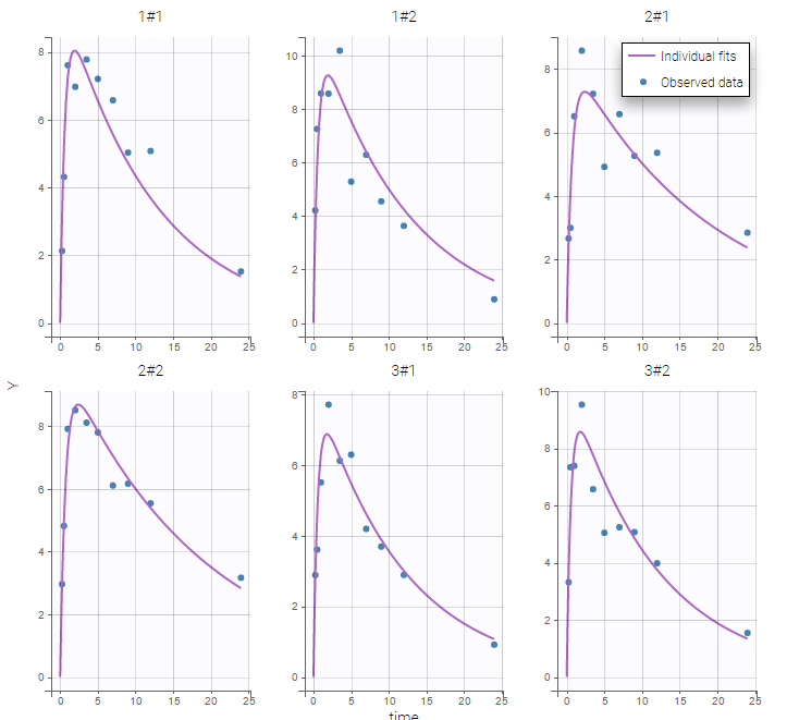
Two important features are proposed in the plots. Firstly, in the individual fits, you can split or merge the occasions. When split is done, the name of the subject-occasion is the name of the subject, #, and the name of the occasion.
 |
 |
|---|
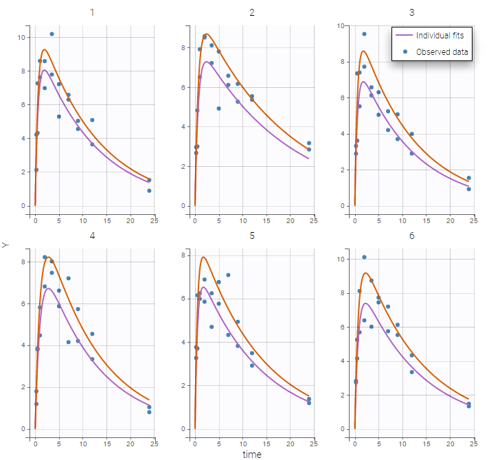
Secondly, you can use the occasion to split the plots
- iov1_Evid_project (data = ‘iov1_Evid_data.txt’, model = ‘lib:oral1_1cpt_kaVk.txt’)
Another way to describe this cross over study is to use EVID=4 as explained in the data set definition. In that example, the EVID creates a washout and another occasion.

Occasions with washout
- iov2_project (data = ‘iov2_data.txt’, model = ‘lib:oral1_1cpt_kaVk.txt’)
The time is increasing in this example, but the dynamical system (i.e. the compartments) is reset when the second period starts. Column EVID provides some information about events concerning dose administration. In particular, EVID=4 indicates that the system is reset (washout) when a new dose is administrated
Monolix automatically proposes to define the treatment periods (between successive resetting) as statistical occasions and introduce IOV, as we did in the previous example. We can display the individual fit by splitting each occasion for each individual
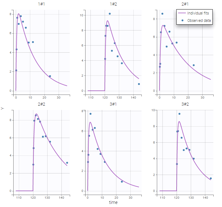
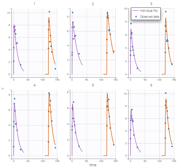
Or by merging the different occasions in a unique plot for each individual:
 Remark: If you are modeling a PK as in this example, the washout implies that the occasions are independent. Thus, the cpu time is much faster as we do not have to compute predictions between occasions.
Occasions without washout
- iov3_project (data = ‘iov3_data.txt’, model = ‘lib:oral1_1cpt_kaVk.txt’)
Multiple doses are administrated to each patient. We consider each period of time between successive doses as a statistical occasion. A column OCCASION is therefore necessary in the data file.
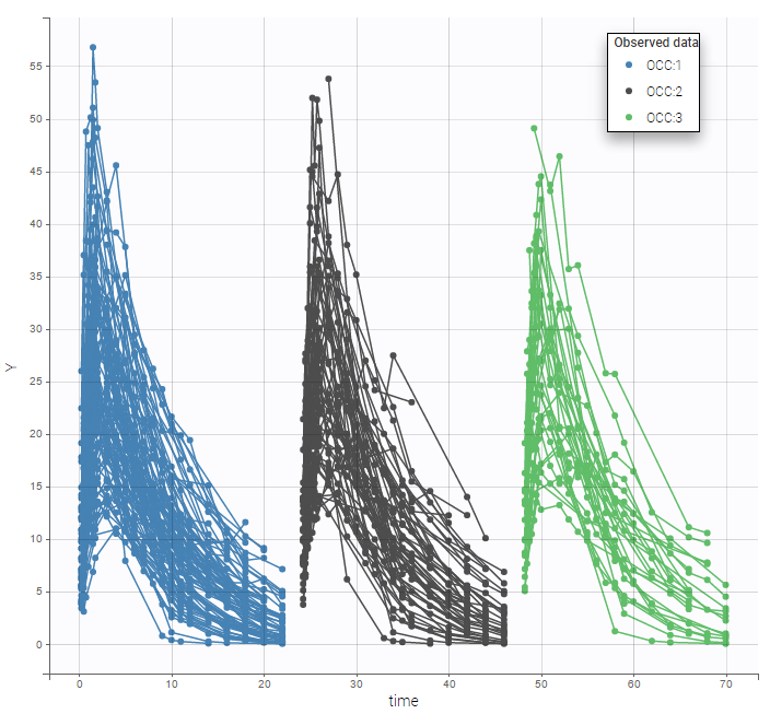
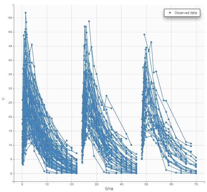 We can color the observed data by their occasion to have a better representation
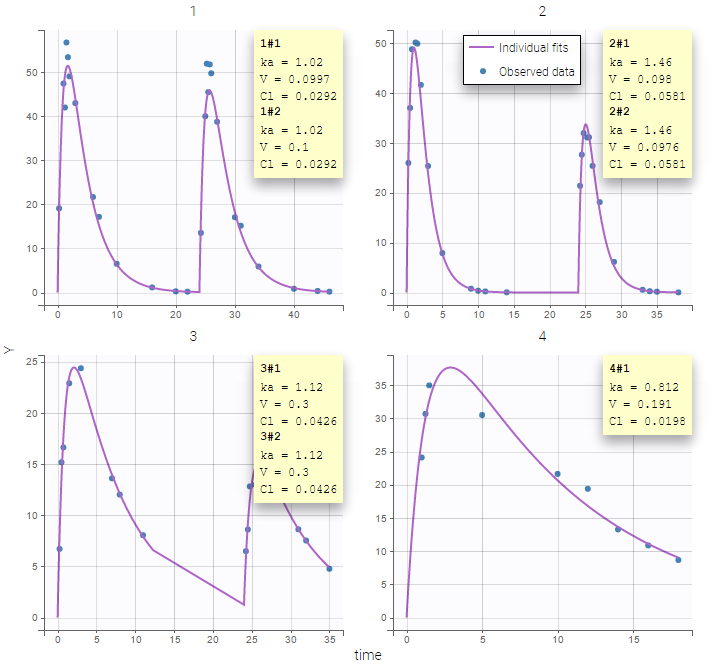
The model for IIV and IOV can then be defined as usual. The plot of individual fits allows us to check that the predicted concentration is now continuous over the different occasions for each individual:
Multiple levels of occasions
- iov4_project (data = ‘iov4_data.txt’, model = ‘lib:oral1_1cpt_kaVk.txt’)
We can easily extend such an approach to multiple levels of variability. In this example, columns P1 and P2 define embedded occasions. They are both defined as occasions:

We then define a statistical model for each level of variability.
