- Introduction
- Mixture of distributions based on a categorical covariate
- Mixture of distributions based on unsupervised classification with a latent covariate
Objectives: learn how to implement a mixture of distributions for the individual parameters.
Projects: PKgroup_project, PKmixt_project
Introduction
Mixed effects models allow us to take into account between-subject variability.
One complicating factor arises when data is obtained from a population with some underlying heterogeneity. If we assume that the population consists of several homogeneous subpopulations, a straightforward extension of mixed effects models is a finite mixture of mixed effects models.
There are two approaches to define a mixture of models:
- defining a mixture of structural models (via a regressor or via the bsmm function) –> click here to go to the page dedicated to this approach,
- introducing a categorical covariate (known or latent). This approach is detailed here.
The second approach assumes that the probability distribution of some individual parameters vary from one subpopulation to another one. The introduction of a categorical covariate (e.g., sex, phenotype, treatment, status, etc.) into such a model already supposes that the whole population can be decomposed into subpopulations. The covariate then serves as a label for assigning each individual to a subpopulation.
In practice, the covariate can either be known or not. If it is unknown, the covariate is called a latent covariate and is defined as a random variable with a user-defined number of modalities in the statistical model. Differences in estimation and diagnosis methods appear to deal with this additional random variable: this difference represents a task of unsupervised classification.
Mixture models usually refer to models for which the categorical covariate is unknown and unsupervised classification is needed.
For the sake of simplicity, we will consider a basic model that involves individual parameters \((\psi_i,1\leq i \leq N)\) and observations \((y_{ij}, i \leq N, 1\leq j \leq n_i)\). Then, the easiest way to model a finite mixture model is to introduce a label sequence \((z_i , 1\leq i \leq N)\) that takes its values in \(\{1,2,\ldots,M\}\) such that \(z_i=m\) if subject i belongs to subpopulation m.
In some situations, the label sequence \((z_i , 1\leq i \leq N)\) is known and can be used as a categorical covariate in the model. If \((z_i)\) is unknown, it can be modeled as a set of independent random variables taking their values in \(\{1,2,\ldots,M\}\) where for \(i=1,2,\ldots, N\), \(P(z_i = m)\) is the probability that individual i belongs to group m. We will assume furthermore that the \((z_i)\) are identically distributed, i.e., \(P(z_i = m)\) does not depend on i for \(m=1, \ldots, M\).
Mixture of distributions based on a categorical covariate
- PKgroup_project (data = ‘PKmixt_data.txt’, model = ‘lib:oral1_1cpt_kaVCl.txt’)
The sequence of labels is known as GROUP in this project and comes from the dataset. It is therefore defined as a categorical covariate that classifies We can then assume, for instance different population values for the volume in the two groups and estimate the population parameters using this covariate model.
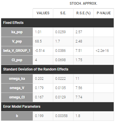
Then, this covariate GROUP can be used as a stratification variable and is very important in the modeling.
Mixture of distributions based on unsupervised classification with a latent covariate
A latent covariate is defined as a random variable, and the probability of each modality is part of the statistical model and is estimated as well. Methods for estimation and diagnosis are different. After the estimation, for each individual the categorical covariate is not perfectly known, only the probabilities of each modality are estimated.
Note also that latent covariates can be useful to model statistical mixtures of populations, but they provide no biological interpretation for the cause of the heterogeneity in the population since they do not come from the dataset.
Latent covariates can not be handled with IOV.
- PKmixt_project (data = ‘PKmixt_data.txt’, model = ‘lib:oral1_1cpt_kaVCl.txt’)
We will use the same data with this project but ignoring the column GROUP (which is equivalent to assuming that the label is unknown). If we suspect some heterogeneity in the population, we can introduce a “latent covariate” by clicking on the grey button MIXTURE.
 It is possible to change the name and the number of modalities of this latent covariate.
Remark: several latent covariates can be introduced in the model, with different number of categories.
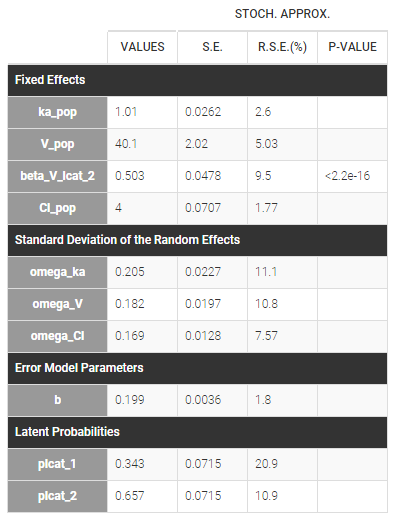
We can then use this latent covariate lcat as any observed categorical covariate. Again, we can assume again different population values for the volume in the two groups by applying it on the volume random effect and estimating the population parameters using this covariate model. Proportions of each group are also estimated, plcat_1 which is the probability to have modality 1:
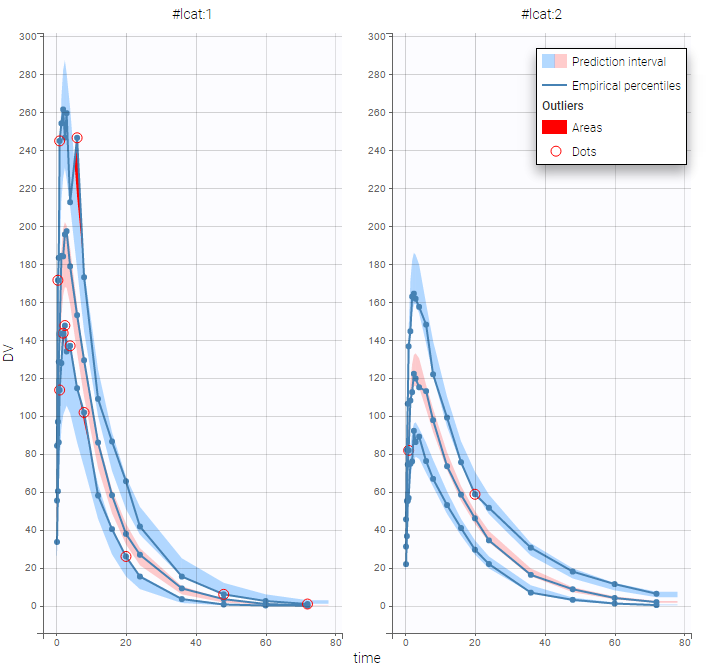
Once the population parameters are estimated, the sequence of latent covariates, i.e. the group to which belongs each subject, can be estimated together with the individual parameters, as the modes of the conditional distributions.
The sequence of estimated latent covariates lcat can be used as a stratification variable. We can for example display the VPC in the 2 groups:
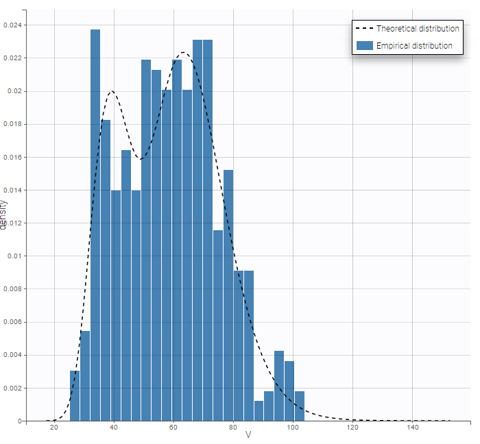
By plotting the distribution of the individual parameters, we see that V has a bimodal distribution