- Introduction
- Conditional distribution
- Conditional mode (EBEs) and conditional mean
- Shrinkage
- Consequences of shrinkage
- How to circumvent shrinkage
- Example
- Conclusion
Introduction
Shrinkage is a phenomenon that appears when the data is insufficient to precisely estimate the individual parameters (EBEs). In that case, the EBEs “shrink” towards the center of the population distribution and do not properly represent the inter-individual variability. This leads to diagnostic plots that may be misleading, either hiding true relationships or inducing wrong ones.
In the diagnostic plots, Monolix uses samples from the conditional distribution as individual parameters, which lead to reliable plots even when shrinkage is present in the model [1]. This method is based on the calculation of the conditional distribution.
Conditional distribution
The conditional distribution is defined for each individual. It represents the uncertainty of the individual’s parameter value, taking the information at hand for this individual into account:
- the observed data for that individual,
- the covariate values for that individual,
- the fact that the individual belongs to the population for which we have already estimated the typical parameter value (fixed effects) and the inter-individual variability (standard deviation of the random effects).
In a mathematical formalism, the conditional distribution is written \(p(\psi_i|y_i;\hat{\theta})\) with \(\psi_i\) the individual parameters for individual \(i\), \(\hat{\theta}\) the estimated population parameters, and \(y_i\) the data (observations) for individual \(i\).
It is not possible to directly calculate the probability for a given \(\psi_i\) (no closed form), but it is possible to obtain samples from the distribution using a Markov-Chain Monte-Carlo procedure (MCMC). This is what is done in the Conditional distribution task.
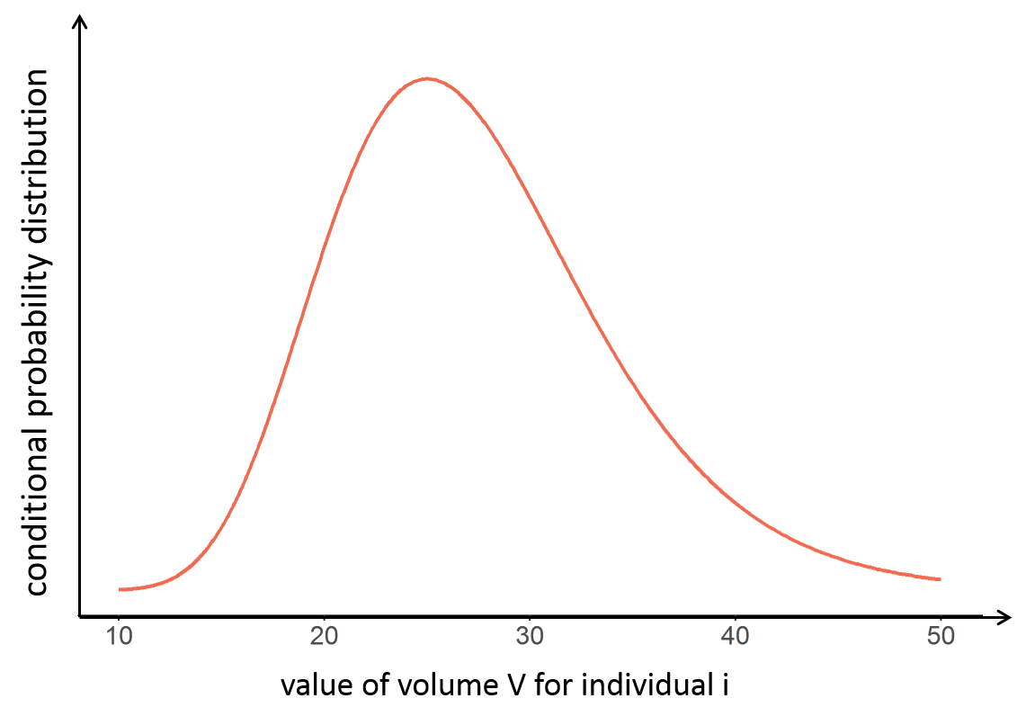
With the following conditional distribution for the volume V of individual i, we see that the most probable value is around 25 L but there is quite some uncertainty: the value could also be 15 or 40 for instance. For visual purpose, we have drawn the distribution as a smooth curve, but remember that the conditional distribution has no explicit expression. One can only obtain samples from this distribution using MCMC.
Conditional mode (EBEs) and conditional mean
It is often convenient to work with a single value for the individual parameters (called an estimator), instead of a probability distribution. Several “summary” values can be used, such as the mode or the mean of the conditional distribution.
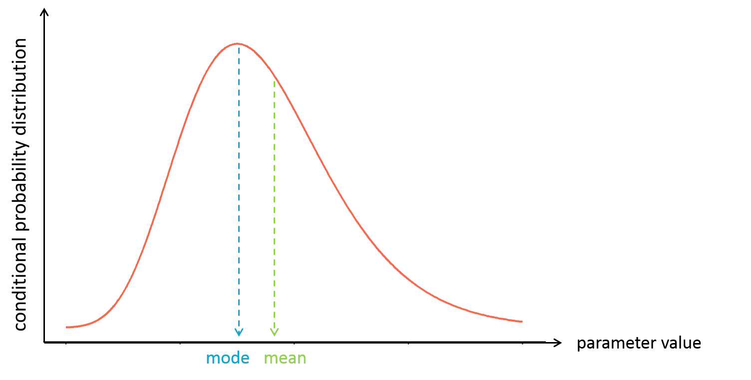
The mode is also called maximum a posteriori or EBE (for empirical bayes estimate). It is often preferred over the mean, because the mode represents the most likely value, i.e the value which has the highest probability.
In Monolix, the mode is calculated via the EBEs task, while the mean is calculated via the Conditional distribution task, as the average of all samples drawn from the conditional distribution.
Once the value of the individual estimator (conditional mode or conditional mean) is known for each individual, one can easily calculate the individual random effects for each individual. For instance for the volume V, that depends on the covariate weight WT:
$$\begin{array}{rl} V_i& = V_{pop}\left(\frac{\textrm{WT}_i}{70}\right)^{\beta}e^{\eta_i} \\ \Rightarrow \quad \eta_i& = \log (V_i) – \log(V_{pop}) – \beta \log \left(\frac{\textrm{WT}_i}{70}\right) \end{array} $$
The individual parameters and individual random effects are used in diagnostic plots. They are used either directly, such as in the Correlation between random effects or Individual parameter versus covariate plots, or indirectly to generate individual predictions, such as in Individual Fits, Observations versus Predictions or Scatter plot of the residuals. But these diagnostic plots can be biased in presence of shrinkage.
Shrinkage
When the individual data brings only few information about the individual parameter value, the conditional distribution is large, reflecting the uncertainty of the individual parameter value. In that case, the mode of the conditional distribution is close to (or “shrinks” to) the mode of the population distribution. If this is the case for all or most of the individuals, all individual parameters end up concentrated around the mode of the population distribution and do not correctly represent the inter-individual variability which has been estimated via the standard deviation parameters (omega parameters in Monolix). This is the shrinkage phenomenon. Shrinkage typically occurs when the data is sparse.
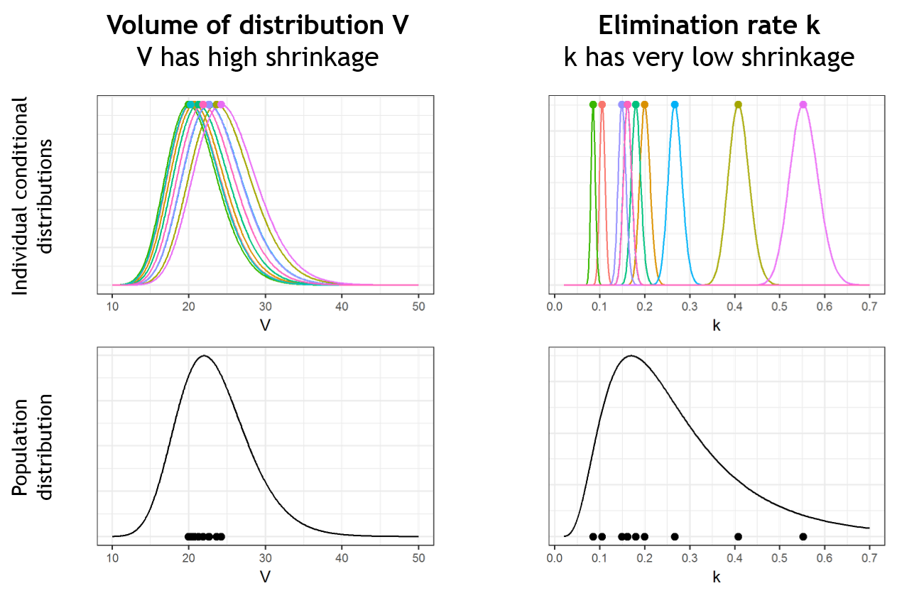
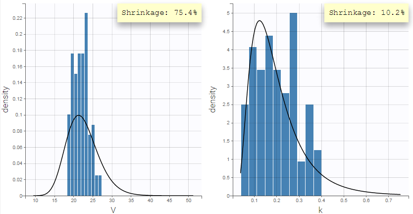
Below we present the example of a parameter V which has a lot of shrinkage and a parameter k with almost no shrinkage. We consider a data set with 10 individuals. In the upper plots, the conditional distributions of each of the 10 individuals are shown. For the volume V, the individual parameter values are uncertain and their conditional distributions are large. When reporting the mode (closed circles) of the conditional distributions on the population distribution (black curve, bottom plots), the modes appear shrunk compared to the population distribution. On the opposite, for k, the conditional distributions are narrow and the modes are well spread over the population distribution. There is shrinkage for V, but not for k.
Pulling the individual parameters of all individuals together, one can overlay the population distribution (black line) with the histogram of individual parameters (i.e conditional modes) (blue bars). This is displayed in the Distribution of the individual parameters plot in Monolix:
The shrinkage phenomenon can be quantified via a shrinkage value for each parameter. In Monolix, the formula for shrinkage has been updated in version 2024 to use the standard deviation instead of the variance in accordance with industry standards.
Starting with Monolix version 2024, shrinkage is calculated from the empirical standard deviation of the random effects \( \textrm{sd}(\eta_i) \) and the estimated standard deviation (the omega population parameter \(\omega\))
$$\eta\textrm{-sh}=1-\frac{\textrm{sd}(\eta_i)}{\omega}$$
In the case of inter occasion variability, shrinkage includes both inter individual and inter occasion variability (the gamma population parameter \(\gamma\))
$$\eta\textrm{-sh}=1-\frac{\textrm{sd}(\eta_i)}{\sqrt{\omega^2 + \gamma^2}}$$
In Monolix versions 2023 and earlier, shrinkage is calculated similarly but with the empirical variance and the estimated variance as:
$$\eta\textrm{-sh}=1-\frac{\textrm{var}(\eta_i)}{\omega^2}$$
Results
In Monolix versions 2023 and earlier, the shrinkage can be displayed in the Distribution of the individual parameters plot, by selecting the “information” toggle.
Starting in Monolix version 2024, shrinkage information is available in several ways:
- Results / Indiv. Results / Cond. Mean [summary] – shrinkage is reported if the Conditional Distribution task has been run
- Results / Indiv. Results / Cond. Mode [summary] – shrinkage is reported if the EBEs task has been run
- In the IndividualParameters folder inside the results folder, there is a file shrinkage.txt
- In reports, using the metric SHRINKAGE in the population or individual parameters table placeholder
- In the plot Distribution of the individual parameters by switching on “information”
- In the plot Distribution of the standardized random effects by switching on “information”
Calculating the shrinkage in R
Starting with Monolix version 2024, there is a method available to directly return the shrinkage information: getEtaShrinkage().
In Monolix version 2023 and earlier, there is no function from the lixoftConnectors to directly get the shrinkage, but you can easily calculate it from the estimated parameters like this for example for parameter V:
population_params <- read.csv("monolix_project/populationParameters.txt")
eta_estimated <- read.csv("monolix_project/IndividualParameters/estimatedRandomEffects.txt")
omega_V <- population_params$value[population_params$parameter=="V"]
eta_V_estimated_mode <- eta_estimated$eta_V_mode
shrinkage_eta_V_estimated_mode <- (1-var(eta_V_estimated_mode)/omega_V^2)*100
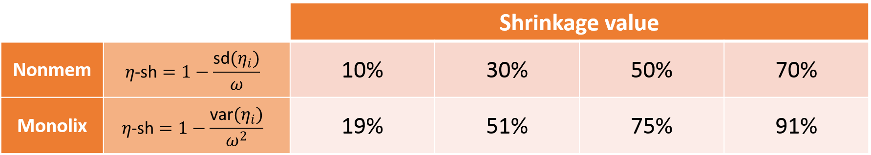
Difference with shrinkage in Nonmem: Note that the Nonmem definition of shrinkage is based on a ratio of standard deviations, while the Monolix definition uses a ratio of variances (which is more common in statistics). Below we provide a “conversion table” which should be read in the following way: a situation that would in Nonmem lead to a shrinkage calculation of 30%, would in Monolix lead to a calculation of shrinkage of around 50%. The Nonmem version of the shrinkage can be calculated from the Monolix shrinkage using the following formula:
$$\eta\textrm{-shNM}=1-\sqrt{1-\eta\textrm{-shMX}}$$
Is it OK to get a negative shrinkage? Yes. In case of no shrinkage, \(var(\eta_i)= \omega^2\) when \(var(\eta_i)\) is calculated on an infinitely large sample. In practice, \(var(\eta_i)\) is calculated on a limited sample related to the number of individuals. Its value can be by chance a little bigger than \(\omega^2\), leading to a slightly negative shrinkage.
Consequences of shrinkage
In case of shrinkage the individual parameters (conditional mode/EBEs or conditional mean) are biased because they do not correctly reflect the population distribution.
As these individual parameters are used in diagnostic plots (in particular the Correlation between random effects and the Individual parameters versus covariates plots) the diagnostic plots can become misleading in presence of shrinkage, either hiding relations or suggesting wrong ones. This complicates the identification of mis-specifications and burdens the modeling process.
Note that the shrinkage of the EBEs has no consequences on the population parameter estimation via SAEM (which doesn’t use EBEs, contrary to FOCE for instance). However the lack of informative data may lead to large standard errors for the population parameters and a slower convergence.
How to circumvent shrinkage
Monolix provides a very efficient solution to circumvent the shrinkage problem, i.e the bias in the diagnostic plots induced by the use of shrunk individual parameters. Instead of using the shrunk conditional mode/EBEs or conditional mean, Monolix uses parameter values randomly sampled from the conditional distribution:

The fact of pooling the random samples of the conditional distribution of all individuals allows us to look at them as if they where sampled from the population distribution. And this is exactly what we want: to have individual parameter values (i.e the samples) that correctly reflect the population distribution.
From a mathematical point of view, one can show that the random samples are an unbiased estimator:
$$p(\psi_i)=\int p(\psi_i|y_i)p(y_i)dy_i=\mathbb{E}_{y_i}(p(\psi_i|y_i))$$
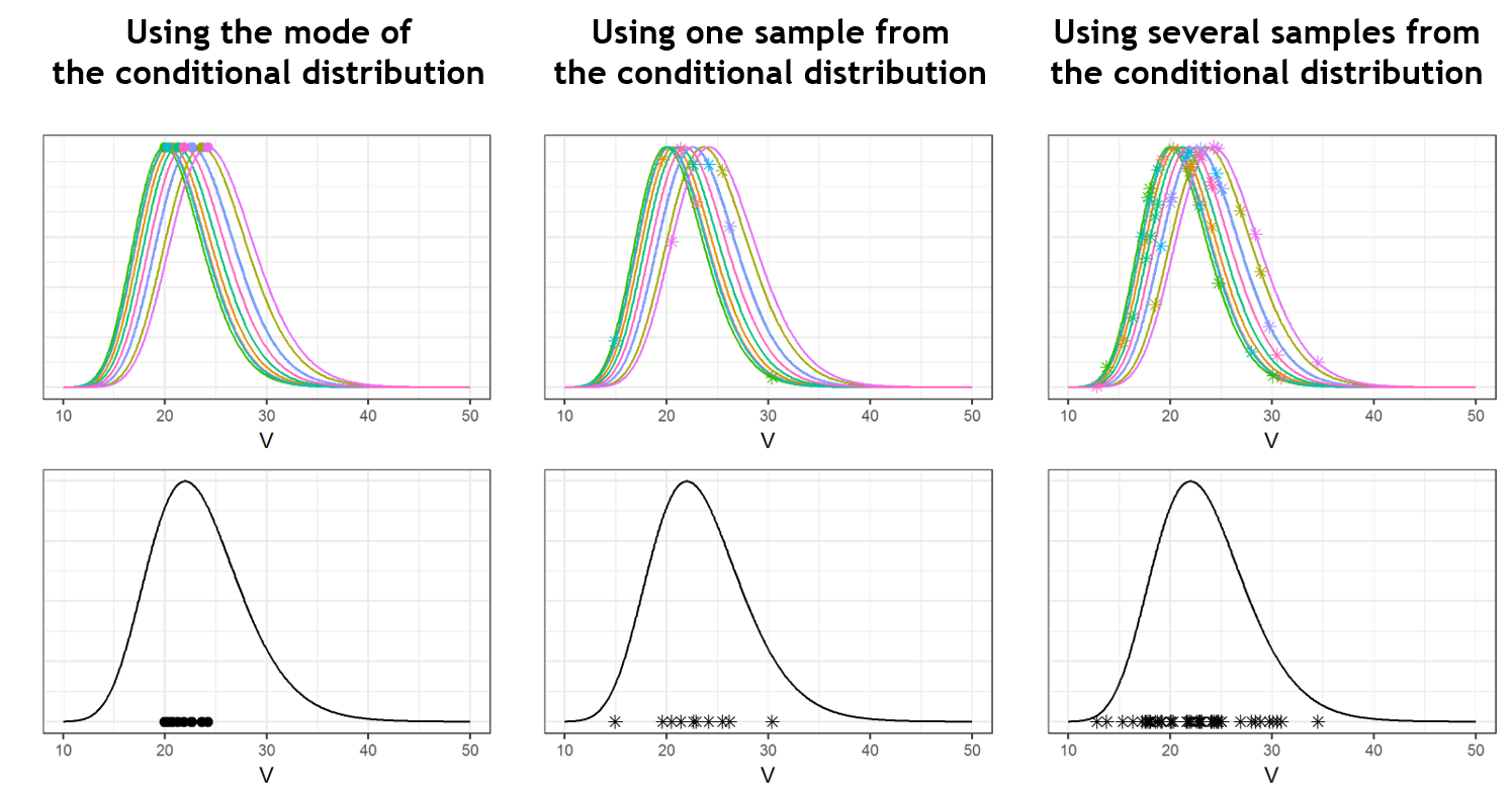
The improvement brought by the random samples from the conditional distributions can be visualized in the following way: while the mode (closed circles) are shrunk, the random samples (stars) spread over the entire population distribution (in black). One can even draw several random sample per individual to increase the informativeness of the diagnostic plots. This is what is done in the MonolixSuite2018R1 version (while MonolixSuite2016R1 uses one sample per individual).
In [1], the authors warrant the use of sampled individual parameters. They demonstrate their usefulness in diagnostic plots via numerical experiments with simulated data. They also show that statistical tests based on these sampled individual parameters are unbiased, the type I error rate is the desired significance level of the test and the probability to detect a mis-specification in the model increases with the magnitude of this mis-specification.
Example
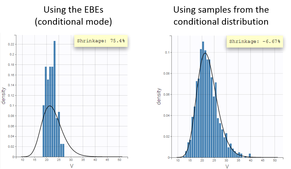
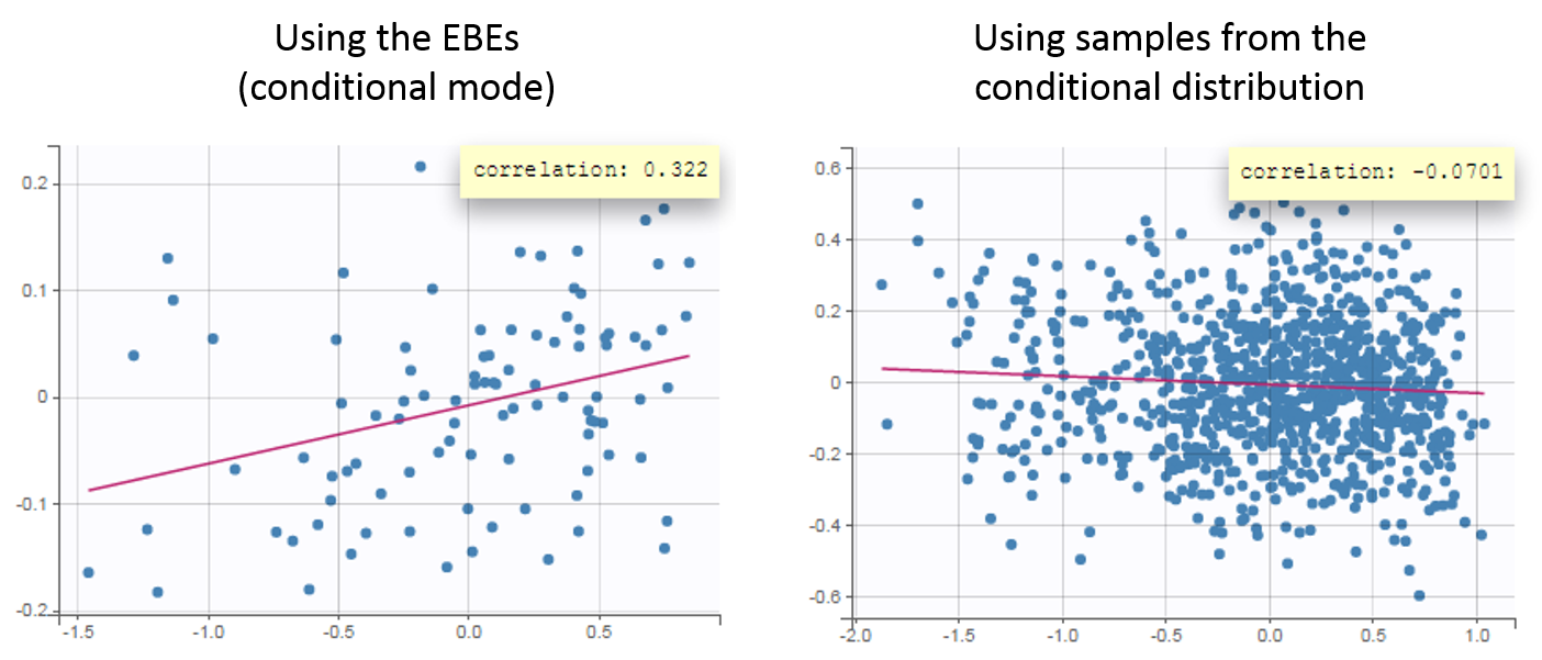
Fitting the sparse Tobramycin data with a (V,k) model leads to a high shrinkage (75%) of the volume V when using the EBEs. On the opposite, when using samples from the conditional distributions of each individual, there is no shrinkage anymore.
The usefulness of using the samples from the conditional distribution can be seen in the Correlation between the random effects plot. Using the EBEs, the plot suggests a positive correlation of about 30% between the volume and the elimination rate. Using the random samples, the plot does not suggest this correlation any more. If the correlation is added to the model, it is estimated small and not significant.
Another example of shrinkage can be seen for the parameter ka in the warfarin data set. In this example, the data is sparse during the absorption phase leading to a large uncertainty of the individual parameter values.
Conclusion
The use of samples from the conditional distribution is a powerful way to avoid the bias due to the shrinkage in the diagnostic plots. This method has been validated mathematically and with numerical experiments.
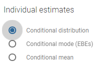
In Monolix, the random samples are used by default in all diagnostic plots, if the Conditional distribution task has been run. The choice of the estimator for the individual parameters can be changed in the Settings tab: