Purpose
These plots display the PWRES (population weighted residuals), the IWRES (individual weighted residuals), and the NPDEs (normalized prediction distribution errors) as scatter plots with respect to the time or the prediction.
The PWRES and NPDEs are computed using the population parameters and the IWRES are computed using the individual parameters. For discrete outputs, only NPDEs are used.
These plots are useful to detect misspecifications in the structural and residual error models: if the model is true, residuals should be randomly scattered around the horizontal zero-line.
Definition
Population Weighted Residuals \(\text{PWRES}_{ij}\)
\(\text{PWRES}_{ij}\) are defined as the normalized difference between the observations and their expected mean. Let \(y_i = (y_{ij}, 1 \leq j \leq n_i)\) be the vector of observations for subject i. The mean of \(y_i\) is the vector \(\mathbb{E}(y_i)=(\mathbb{E}(f(t_{ij};\psi_i), 1 \leq j \leq n_i)\). Let \( \textrm{V}_i\) be the \(n_j \times n_j\) variance-covariance matrix of \(y_i\). Then, the ith vector of the population weighed residuals \( \text{PWRES}_i = \{\text{PWRES}_{ij}, 1\leq j \leq n_i\} \) is defined by
$$\text{PWRES}_i = V_i^{-1/2}(y_i-\mathbb{E}(y_i))$$
The population residuals \((y_i-\mathbb{E}(y_i))\) are correlated within each individual. The population weighted residuals PWRES standardize and decorrelate the population residuals using the model-predicted variance-covariance matrix of observations \(V_i\).
\(\mathbb{E}(y_i) \) and \(V_i\) are not known in practice but are estimated empirically by Monte-Carlo simulation without any approximation of the model. In the formula above, \(y_i\) represents the observations from the dataset. \(\mathbb{E}(y_i)\) is calculated as the mean of simulated observations using individual parameters sampled from the population distribution to obtain the model prediction plus a sample from the residual error model. The number of simulated observations depends on the Plot task setting “Number of simulations”. \(V_i\) is calculated on the same simulated observations.
When the PWRES are plotted w.r.t the model prediction, the population prediction popPred (i.e with random effects eta equal to zero but keeping the covariate effects) are used on the x-axis.
Individual weighted residuals \(\text{IWRES}_{ij}\)
\(\text{IWRES}_{ij}\) are estimates of the standardized residual (\(\epsilon_{ij}\)) based on individual predictions, with \(g\) the function defining the residual error model:
$$\text{IWRES}_{ij} = \dfrac{ y_{ij}-f(t_{ij};\hat{\psi}_i)}{g(t_{ij};\hat{\psi}_i)}$$
If the residual errors are assumed to be correlated, the individual weighted residuals can be decorrelated by multiplying each individual vector \(\text{IWRES}_i = (\text{IWRES}_{ij} ; 1\leq j\leq n_i)\) by \(\hat{\text{R}}_i^{-1/2}\), where \(\hat{\text{R}}_i\) is the estimated correlation matrix of the vector of residuals \((\epsilon_{ij}; 1\leq j \leq n_i)\).
When the IWRES are plotted w.r.t the model prediction, the individual prediction using the conditional mode (EBEs), conditional mean or samples from the conditional distribution is used, depending on the choice of the “Individual estimates” in the settings panel on the right.
Normalized prediction distribution errors \(\text{NPDE}_{ij}\)
\(\text{NPDE}_{ij}\) are a nonparametric version of \(\text{PWRES}_{ij}\) based on a rank statistic. For any (i,j), let \(\text{F}_{ij} = \text{F}_{\text{PWRES}_{ij}}(\text{PWRES}_{ij})\) where \(\text{F}_{\text{PWRES}_{ij}}\) is the cumulative distribution function (cdf) of \(\text{PWRES}_{ij}\). NPDEs are then obtained from \(\text{F}_{ij}\) by applying the inverse of the standard normal cdf \(\Phi\).
In practice, one simulates a large number \(K\) of simulated data set \(y^{(k)}\) using the model, and estimate \(\text{F}_{ij}\) as the fraction of simulated data below the original data, i.e:
$$\hat{\text{F}}_{ij}=\frac{1}{K}\sum_{k=1}^K 1_{y_{ij}^{(k)}\leq y_{ij}^{\text{obs}}}$$
By definition, the distribution of \(\text{F}_{ij}\) is uniform on [0,1], we thus rather use \(\Phi^{-1}(\text{F}_{ij})\), which follows a standard normal distribution (with \(\Phi\) the cdf of the standard normal distribution). NPDEs are defined as an empirical estimation of \(\Phi^{-1}(\text{F}_{ij})\), i.e \(\text{NPDE}_{ij}=\Phi^{-1}(\hat{\text{F}}_{ij})\).
When the NPDE are plotted w.r.t the model prediction, the population prediction popPred (i.e with random effects eta equal to zero but keeping the covariate effects) are used on the x-axis.
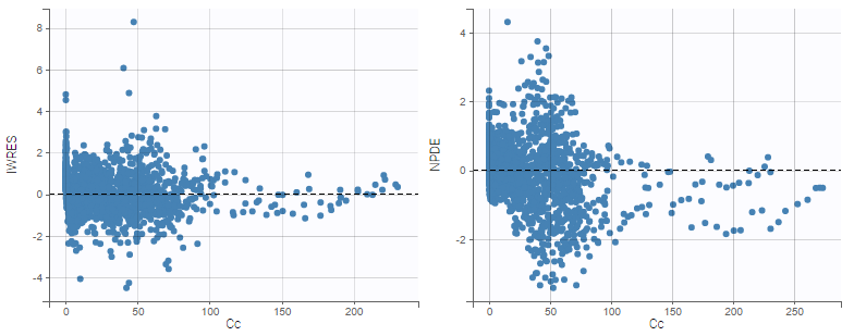
Below is a correspondence table of the Nonmem and Monolix terms used for residuals:
For count and categorical data:
FAQ: Is there no CWRES in Monolix? No, PWRES are given instead. They are defined with the same formula but are obtained with simulations rather than FOCE approximation, so without any approximation of the model. The PWRES in Monolix are equivalent to the EWRES in Nonmem.
Examples
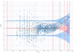
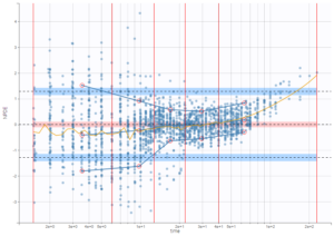
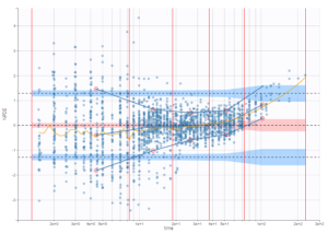
In the following example, the parameters of a two-compartment model with iv unfusion and linear elimination are estimated on the remifentanil data set. One can see the PWRES, the IWRES and the NPDE w.r.t. the time (on top), and the prediction (at the bottom).
Since the points are clearly scattered unevenly around the horizontal zero-line, these plots suggest a misspecifcation of the structural model.
The corresponding distributions can be seen on this page.

It is possible to select some of the subplots to focus on, with the panel Subplots in Settings:

Presets
A number of element can be overlaid or hidden from the plots in the panel Display. Only the horizontal zero-line, representing the theoretical mean, is always displayed. Two presets with predefined selections of displayed elements are available: the first one called “Scatter” hides all elements except the points for residuals, while the second called “VPC” displays instead empirical and predicted percentiles for the residuals as lines, as well as prediction intervals as colored areas. This figure is detailed below.
 |
 |
|---|
Predictive checks
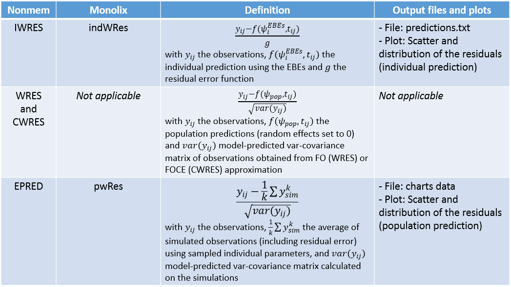
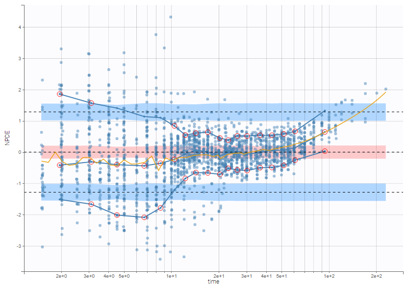
The preset “VPC” displays prediction intervals for the median, 10th and 90th percentiles, obtained with simulations of the residuals, as well as the empirical percentiles to compare the behavior of the model to the data. Residual points are hidden, but the trend is represented with a spline interpolation.
Misspecification in the structural model, the error model, and the covariate model can be detected by discrepancies between the observed percentiles and their prediction intervals, as can be seen for example on the plots of IWRES vs time and NPDE vs time below, with log-scale on the x-axis. Population residuals greatly depart from the data at all time points, while individual residuals show better predictions for low times only.
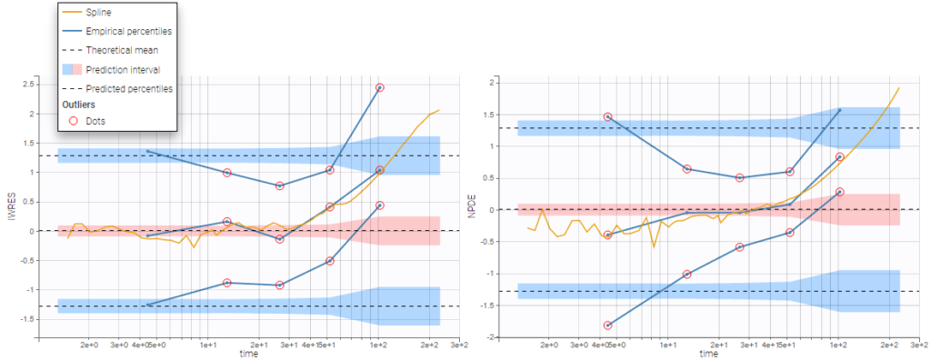
Outliers (empirical percentiles outside the prediction intervals) can be marked with red points or red areas:
Comparing PWRES and NPDEs
NPDEs are quite similar to PWRES, but are simulation-based, and therefore account for the heterogeneity in study design by comparing the observations with their own distribution. NPDEs are thus displayed by default rather than PWRES.

Comparing IWRES and NPDEs
The IWRES are based on individual predictions, therefore the values on the X axis with respect to predictions are not the same as for NPDEs and PWRES, as can be seen on the plots below. If the tasks EBEs and Conditional distribution have been run, several different individual estimates are available to be used for the individual predictions. The next section shows how to choose the estimates.
Preventing shrinkage in IWRES
The individual estimates used to compute the IWRES can be chosen in the Display panel:

By default, the individual estimates are drawn from the conditional distributions rather than coming from usual estimators such as conditional modes (EBEs) or conditional means. This choise is recommended in order to prevent shrinkage, a phenomenon that occurs when the individual data are not sufficiently informative with respect to one or more parameters. If overfitting occurs, IWRES computed from biased estimators might thus shrink toward 0.
Highlight
Hovering on a point highligths all the points from the same individual in yellow on all plots, and reveals the corresponding subject id and time. If the individual estimates selected in Display are the simulated condition distribution, each observation corresponds to a set of IWRES computed from a set of simulated individual parameters. When the observation is hovered, the points from this set are indicated with a bigger diameter.

If the individual estimates selected in Display are condition modes (EBEs) or conditional means, there is only one residual per observation, and all points corresponding to the same individual are linked with segments to visualize the time chronology.

Binning
As for VPC, data binning used to compute percentiles can be changed. Several strategies exist to segment the data: equal-width binning, equal-size binning, and a least-squares criterion. The number of bins can also be either set by the user, or automatically selected to obtain a good trade off.
On the three figures below where NPDEs are displayed with respect to log-scaled time, 5 bins are selected with equal width on the left, equal size in the center, and the least-squares criteria on the right. Observations are overlaid in light purple to visualize the data density in each bin. Equal width in particular shows low density for some bins, and result in a less informative plot for low times were data density is high.
 |
 |
 |
|---|
On the figure below, the number of bins for least-squares criteria is automatically set, allowing a more precise display.
Censored data
The residuals for censored data appear in a different color. They are by default based on simulated observations that take into account the censoring interval.
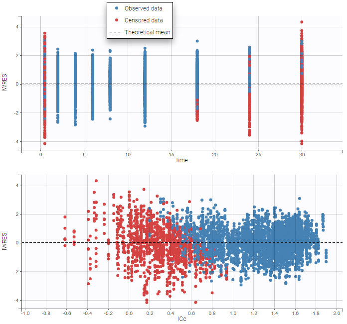
An option available in the panel “Display” can be used to select the method of calculation for the residuals corresponding to censored data: either based on simulated observations (by default), or based on LOQ (values from the observation column in the dataset).

Discrete data
For categorical or count data, only NPDEs are used. Here again, NPDEs correspond to the rank of each observation among a set of simulations based on the model. However, to prevent problems with discrete values, both observations and simulations are slightly perturbed with a uniform distribution before computing the ranks.
Settings
- Subplots
- Residuals
- Population residuals: Add/remove scatterplots for PWRES. Hidden by default.
- Individual residuals: Add/remove scatterplots for IWRES, using the individual parameter estimated using the conditional mode or the conditional mean. By default, individual parameters come from the conditional mode estimation.
- NPDE: Add/remove scatterplots for NPDE.
- X-axis
- time: Add/remove the scatterplots w.r.t. the time.
- prediction: Add/remove the scatterplots w.r.t. the prediction.
- Residuals
- Display
- Presets: apply the preselections of elements for scatter plots or VPC
- Residuals: Add/remove observed data.
- Censored data: Add/remove BLQ data (with a different color) if present.
- Empirical percentiles: Add/remove empirical percentiles for the 10%, 50% and 90% quantiles.
- Predicted percentiles: Add/remove theoretical percentiles for the 10% and 90% quantiles.
- Prediction interval: Add/remove prediction intervals given by the model for the 10% and 90% quantiles (in blue) and the 50% quantile (in pink), with user-defined level (by default, 90).
- Outliers: Add/remove dots or areas to mark outliers.
- Individual estimates: Choose the individual estimates among conditional modes (EBEs), conditional means (computed with SAEM), or simulated parameters from the conditional distributions.
- Calculations – linear interpolation: Choose the display for prediction intervals: by default linear interpolation is used, otherwise the display is piecewise.
- Calculations – Use censored data: Choose the display for censored data: by default simulated BLQ observations are used, otherwise the LOQ from the observation column in the data set can be used.
- Visual cues: Add/remove spline interpolation.
- Bins
- Bin values: Add/remove vertical lines on the scatterplots to indicate the bins.
- Binning criteria: Choose the bining criteria among equal width (default), equal size or least-squares.
- Number of bins: Choose a fixed number of bins or a range, with the range for the number of data points per bin.