Population parameter estimation using SAEM

• Purpose
• Calculations: the SAEM algorithm
• Running the population parameter estimation task
  • Overview
  • Dependencies between tasks
  • The convergence indicator
  • The simulated annealing
  • Methods for parameters without variability
  • Other estimation methods: Fixing population parameters or Bayesian estimation
• Outputs
  • In the graphical user interface
  • In the output folder
• Settings
• Good practices, troubleshooting and tips

Purpose

The estimation of the population parameters is the key task in non-linear mixed effect modeling. In Monolix, it is performed using the Stochastic Approximation Expectation-Maximization (SAEM) algorithm [1]. SAEM has been shown to be extremely efficient for both simple and a wide variety of complex models: categorical data [2], count data [3], time-to-event data [4], mixture models [5–6], differential equation based models, censored data [7], … The convergence of SAEM has been rigorously proven [1] and its implementation in Monolix is particularly efficient. No other algorithms are available in Monolix.

Calculations: the SAEM algorithm

 

 

Running the population parameter estimation task

Overview

The pop-up window which permits to follow the progress of the task is shown below. The algorithm starts with a small number (5 by default) of burn-in iterations for initialization which are displayed in the following way: (note that this step can be so fast that it is not visible by the user)

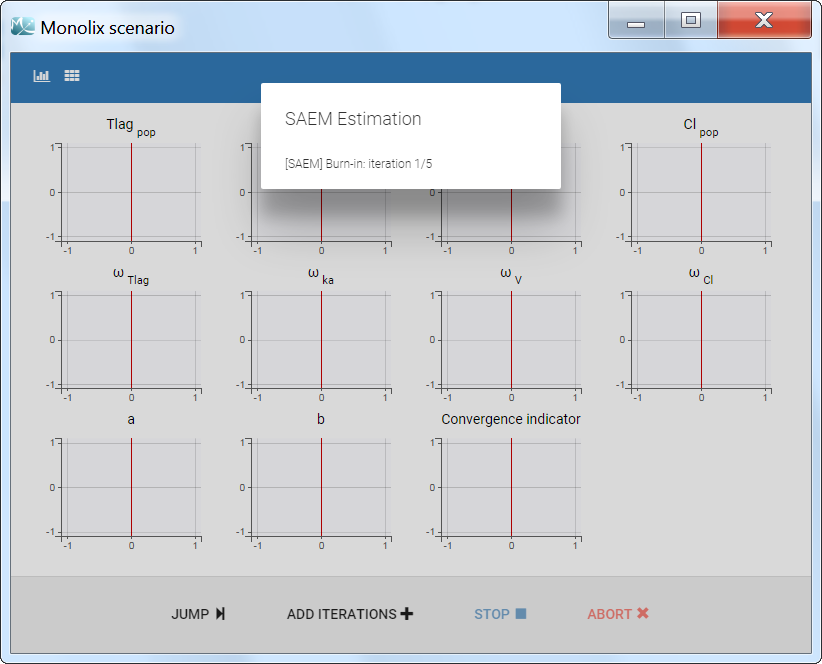
Afterwards, the evolution of the value for each population parameter over the iterations of the algorithm is displayed. The red line marks the switch from the exploratory phase to the smoothing phase. The exact value at each iterations can be followed by hovering over the curve (as for Cl_pop below). The convergence indicator (in purple) helps to detect that convergence has been reached (see below for more details).

 

Dependencies between tasks

The “Population parameter” estimation task must be launched before running any other task. To skip this task, the user can fix all population parameters. If all population parameters have been set to “fixed”, the estimation will stop after a single iteration and allow the user to continue with the other tasks.

The convergence indicator

The convergence indicator (also sometimes called complete likelihood) is defined as the joint probability distribution of the data and the individual parameters and can be decomposed using Bayes law:

\(\sum_{i=1}^{N_{\text{ind}}}\log\left(p(y_i, \phi_i; \theta)\right)=p(y_i| \psi_i; \theta)p(\psi_i; \theta)\)

Those two terms have an analytical expression and are easy to calculate, using as \(\phi_i\) the individual parameters drawn by MCMC for the current iteration of SAEM. This quantity is calculated at each SAEM step and is useful to assess the convergence of the SAEM algorithm.
The convergence indicator aggregates the information from all parameters and can serve to detect if the SAEM algorithm has already converged or not. When the indicator is stable, that is it oscillates around the same value without drifting, then we can be pretty confident that the maximum likelihood has been achieved. The convergence indicator is used, among other measures, in the auto-stop criteria to switch from the exploratory phase to the smoothing phase.
Note that the likelihood (i.e the objective function) \(\sum_{i=1}^{N_{\text{ind}}}\log\left(p(y_i; \theta)\right)\) cannot be computed in closed form because the individual parameters \(\phi_i\) are unobserved. It requires to integrate over all possible values of the individual parameters. Thus, to estimate the log-likelihood an importance sampling Monte Carlo method is used in a separate task (or an approximation is calculated via linearization of the model).

The simulated annealing

The simulated annealing option (setting enabled by default) permits to keep the explored parameter space large for a longer time (compared to without simulated annealing). This allows to escape local maximums and improve the convergence towards the global maximum.
In practice, the simulated annealing option constrains the variance of the random effects and the residual error parameters to decrease by maximum 5% (by default – the setting “Decreasing rate” can be changed) from one iteration to the next one. As a consequence, the variances decrease more slowly:

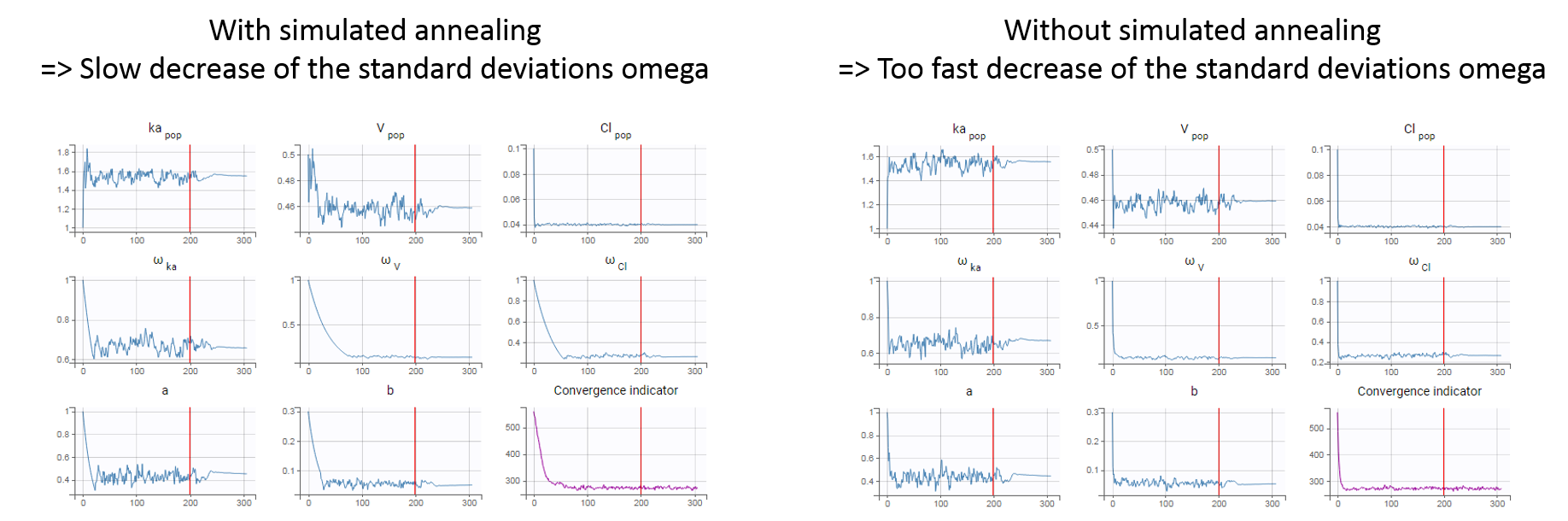
The size of the parameter space explored by the SAEM algorithm depends on individual parameters sampled from their conditional distribution via Markov Chain Monte Carlo. If the standard deviation of the conditional distributions is large, the individual parameters sampled at iteration k can be quite far away from those at iteration (k-1), meaning a large exploration of the parameter space. The standard deviation of the conditional distribution depends on the standard deviation of the random effects (population parameters ‘omega’). Indeed, the conditional distribution is \(p(\psi_i|y_i;\hat{\theta})\) with \(\psi_i\) the individual parameters for individual \(i\), \(\hat{\theta}\) the estimated population parameters, and \(y_i\) the data (observations) for individual \(i\). The conditional distribution thus depends on the population parameters, and the larger the population parameters ‘omega’, the larger the standard deviation of the conditional distribution. That’s why we want to keep large ‘omega’ values during the first iterations.

Methods for the parameters without variability

Parameters without variability are not estimated in the same way as parameters with variability. Indeed, the SAEM algorithm requires to draw parameter values from their marginal distribution, which exists only for parameters with variability.
Several methods can be used to estimate the parameters without variability. By default, these parameters are optimized using the Nelder-Mead simplex algorithm (Matlab’s fminsearch method). Other options are also available in the SAEM settings:

• No variability (default): optimization via Nelder-Mead simplex algorithm
• Add decreasing variability: an artificial variability (i.e random effects) is added for these parameters, allowing estimation via SAEM. The variability starts at omega=1 and is progressively decreased such that at the end of the estimation process, the parameter has a variability of 1e-5. The decrease in variability is exponential with a rate based on the maximum number of iterations for both the exploratory and smoothing phases. Note that if the autostop is triggered, the resulting variability might me higher.
• Variability at the first stage: during the exploratory phase of SAEM, an artificial variability is added and progressively forced to 1e-5 (same as above). In the smoothing phase, the Nelder-Mead simplex algorithm is used.

Depending on the specific project, one or the other method may lead to a better convergence. If the default method does not provide satisfying results, it is worth trying the other methods. In terms of computing time, if all parameters are without variability, the first option will be faster because only the Nelder-Mead simplex algorithm will be used to estimate all the fixed effects. If some parameters have random effects, the first option will be slower because the Nelder-Mead and the SAEM algorithm are computed at each step. In that case the second or third option will be faster because only the SAEM algorithm will be required when the artificial variability is added.

Alternatively, the standard deviation of the random effects can be fixed to a small value, for instance 5% for log-normally distributed parameters. (See next section on how to enforce a fixed value). With this method, the SAEM algorithm can be used, and the variability is kept small.

 

Other estimation methods: fixing population parameters or Bayesian estimation

Instead of the default estimation method with SAEM, it is possible to fix a population parameter, or set a prior on the estimate and use Bayesian estimation. This page gives details on these methods and how to use them.

 

 

Outputs

In the graphical user interface

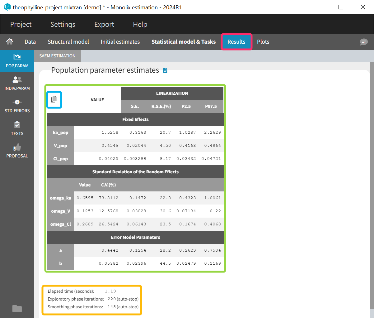
The estimated population parameters are displayed in the POP.PARAM section of the RESULTS tab. Fixed effects names are “*_pop”, the standard deviation of the random effects “omega_*”, parameters of the error model “a”, “b”, “c”, the correlation between random effects “corr_*_*” and parameters associated to covariates “beta_*_*”. The standard deviation of the random effects is also expressed as coefficient of variation (CV) – a feature present in versions Monolix 2023 or above. The CV calculation depends on the parameter distribution:

• lognormal: \(CV=100*\sqrt{exp(\omega_p^2) -1}\)
• normal: \(CV=100*\frac{\omega_p}{p_{pop}}\)
• logitnormal and probitnormal: the CV is computed by Monte-Carlo. 100000 samples X are drawn from the distribution (defined by \(\omega_p\) and \(p_{pop}\)) and the CV is calculated as the ratio of the sample standard deviation over the sample mean: \(CV=100*\frac{sd(X)}{mean(X)}\)

When you run the “Standard errors” task, then the population parameter table contains also the standard error (s.e) and relative standard error (r.s.e). Note that the CV% represents the inter-individual variability, while the RSE% represents the uncertainty on the estimated parameters.

Starting from version 2024, alongside the standard errors, the upper and lower percentiles, here P2.5 and P97.5 of the confidence interval with level 1−\( \alpha\) are computed for population parameters. This calculation depends on the execution of the “Standard errors” task, as it relies on the standard error of the respective parameter. In order to take into account the boundaries of the parameters (e.g omega or V_pop cannot be negative), the SE is transformed into the gaussian domain, the CI in gaussian domain is calculated assuming a normal distribution and finally the CI is backtransformed. Its transformation is determined by the type of parameter and its distribution assumption:

• Normal distributed parameters: \(CI_{1-\alpha} (\theta _{pop})=[\theta_{pop} + q_{\alpha /2}\times s.e.(\theta_{pop}), ~\theta_{pop} + q_{1 – \alpha /2}\times s.e.(\theta_{pop})]\). This applies for typical values (fixed effects) of normally distributed parameters and covariate effects (betas).
• Lognormal distributed parameters: \(CI_{1-\alpha} (\theta _{pop})=[\exp(\mu_{pop} + q_{\alpha /2}\times s.e.(\mu_{pop})), ~\exp(\mu_{pop} + q_{1 – \alpha /2}\times s.e.(\mu_{pop}))]\),  where \( \mu_{pop} = \ln(\theta_{pop})\). This applies to typical values (fixed effects) of lognormally distributed parameters, standard deviations of the random effects (omegas), and error model parameters.
• Logitnormal distributed parameters: \(CI_{1-\alpha} (\theta _{pop})=[logit^{-1}(\mu_{pop} + q_{\alpha /2}\times s.e.(\mu_{pop})), ~logit^{-1}(\mu_{pop} + q_{1 – \alpha /2}\times s.e.(\mu_{pop}))]\),  where \( \mu_{pop} = logit(\theta_{pop})\). This applies to typical values (fixed effects) of logit-normally distributed parameters and correlation parameters.

where \(q_{\alpha /2}\) is the quantile of order \( \alpha /2\) for a standard normal distribution. The confidence interval level \( \alpha\) can be modified in the settings of the “Standard errors” task within the Statistical Model & Tasks tab by clicking on the wrench icon.

Information about the SAEM task performance are below the table (orange frame):

• The total elapsed time for this task
• The number of iterations in the exploratory and smoothing phases, along with a message that indicates whether the convergence has been reached (“auto-stop”), or if the algorithm arrived at the maximum number of iterations (“stopped at the maximum number of iterations/auto-stop criteria have not been reached”) or if it was stopped by the user (“manual stop”). (for Monolix versions 2021 or above)

A “Copy table” icon on the top of the table allows to copy it in Excel, Word, etc. The table format and display is kept.

Starting from version 2024R1, if categorical covariate effects are included in the statistical model, a “Display fixed effects by category” toggle allows to add a section named “Fixed effects by category” in the table, with the values of the typical population parameters in each category of the categorical covariates and their SEs, RSEs and confidence intervals.

In the output folder

After having run the estimation of the population parameters, the following files are available:

• summary.txt: contains the estimated population parameters (and the number of iterations in Monolix2021R1), in a format easily readable by a human (but not easy to parse for a computer)
• populationParameters.txt: contains the estimated population parameters (by default in csv format), including the CV.
• populationParametersByGroups.txt: contains the estimated population parameters by categories of categorical covariates included in the statistical model. This file is not generated if there are no categorical covariate effects.
• predictions.txt: contains for each individual and each observation time, the observed data (y), the prediction using the population parameters and population median covariates value from the data set (popPred_medianCOV), the prediction using the population parameters and individual covariates value (popPred), the prediction using the individual approximate conditional mean calculated from the last iterations of SAEM (indivPred_SAEM) and the corresponding weighted residual (indWRes_SAEM).
• IndividualParameters/estimatedIndividualParameters.txt: individual parameters corresponding to the approximate conditional mean, calculated as the average of the individual parameters sampled by MCMC during all iterations of the smoothing phase. When several chains are used (see project settings), the average is also done over all chains. Values are indicated as *_SAEM in the file.
  Parameters without variability: 
  • method “no variability” or “variability at the first stage”: *_SAEM represents the value at the last SAEM iteration, so the estimated population parameter plus the covariate effects. In absence of covariate, all individuals have the same value.
  • method “add decreasing variability”: *_SAEM represents the average of all iterations of the smoothing phase. This value can be slightly different from individual to individual, even in te absence of covariates.
• IndividualParameters/estimatedRandomEffects.txt: individual random effects corresponding to the approximate conditional mean, calculated using the last estimations of SAEM (*_SAEM).
  For parameters without variability, see above.

More details about the content of the output files can be found here.

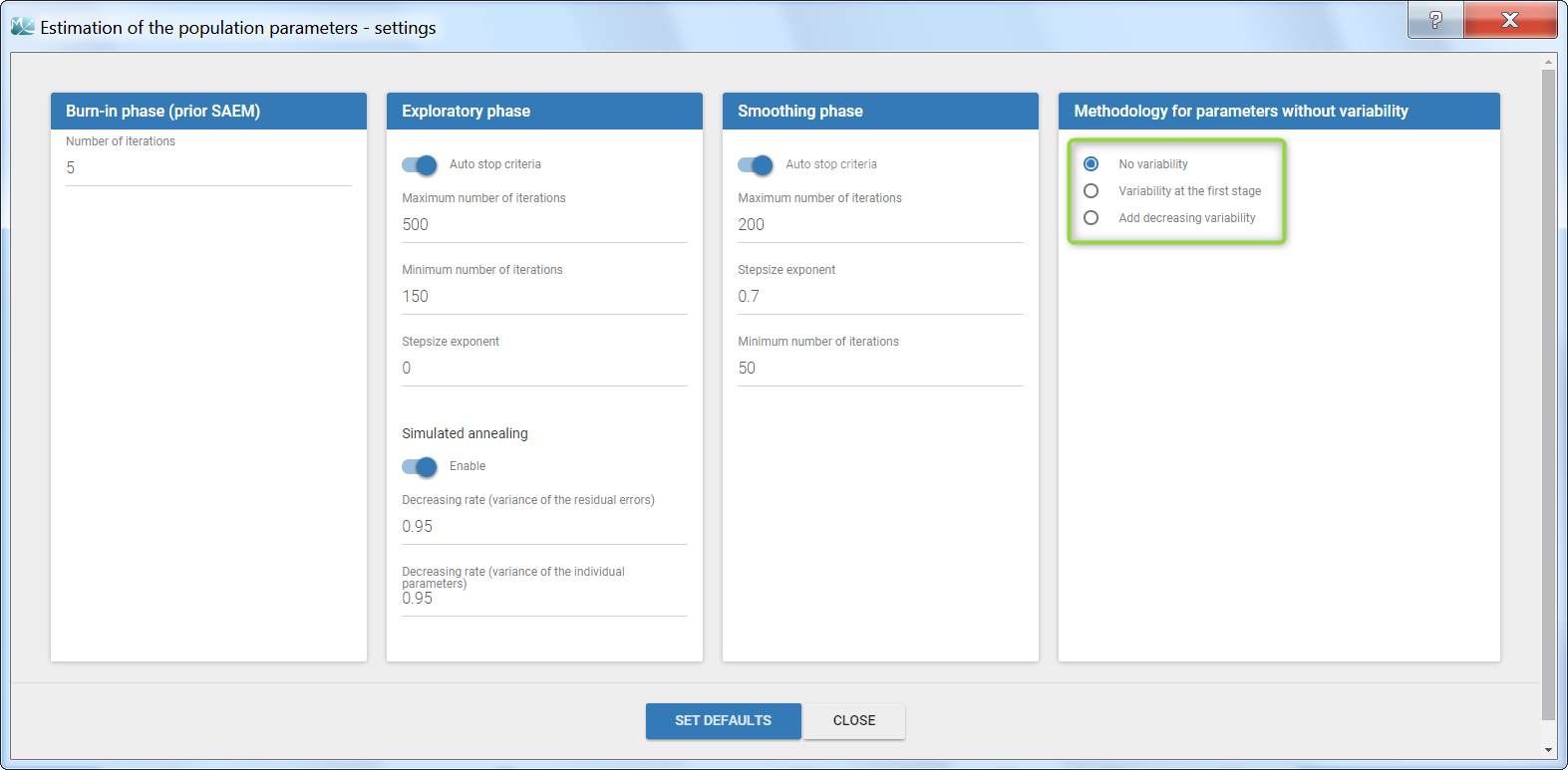
Settings

The settings are accessible through the interface via the button next to the parameter estimation task.

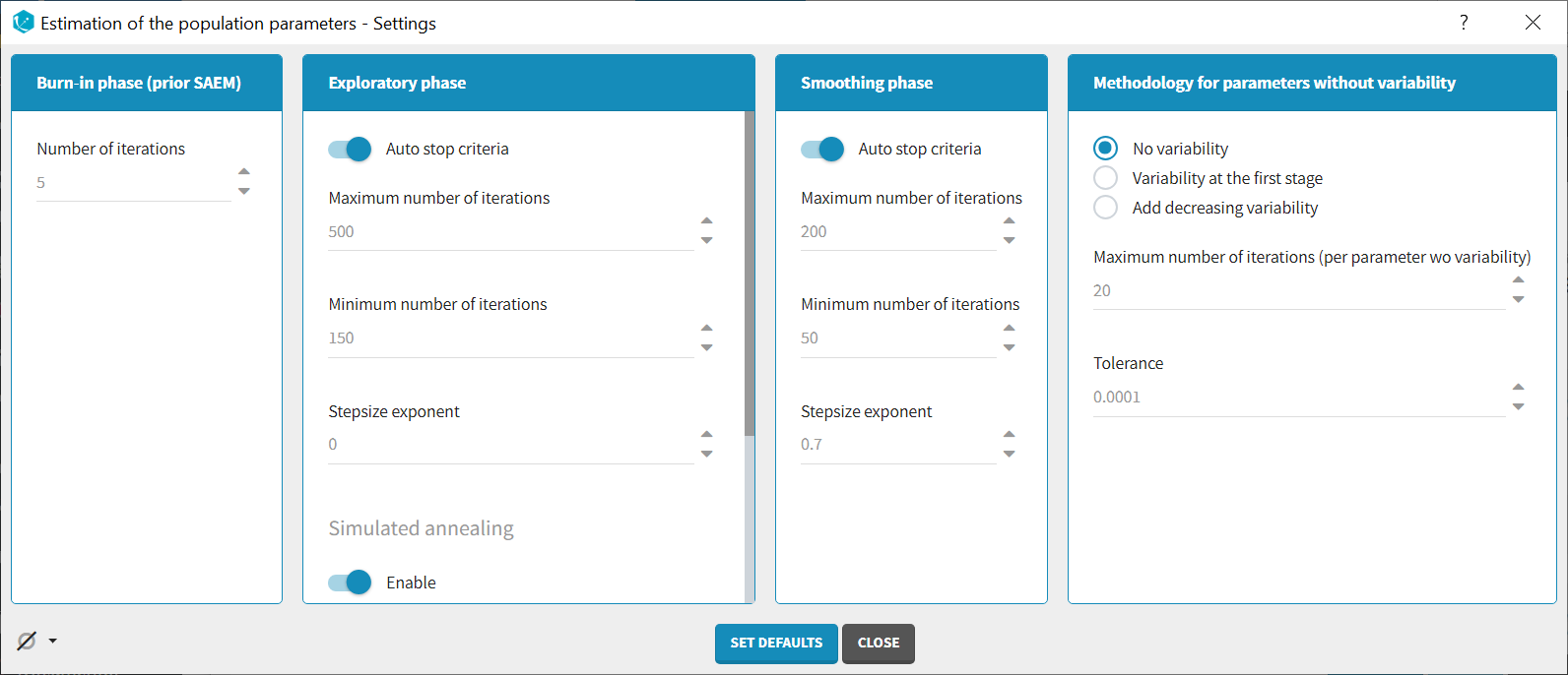
Burn-in phase:

The burn-in phase corresponds to an initialization of SAEM: individual parameters are sampled from their conditional distribution using MCMC using the initial values for the population parameters (no update of the population parameter estimates).
Note: the meaning of the burn-in phase in Monolix is different to what is called burn-in in Nonmem algorithms.

• Number of iterations (default: 5): number of iterations of the burn-in phase

Exploratory phase: 

• Auto-stop criteria (default: yes): if ticked, auto-stop criteria are used to automatically detect convergence during the exploratory phase. If convergence is detected, the algorithm switches to the smoothing phase before the maximum number of iterations. The criteria take into account the stability of the convergence indicator, omega parameters and error model parameters.
• Maximum number of iterations (default: 500, if auto-stop ticked): maximum number of iterations for the exploratory phase. Even if the auto-stop criteria are not fulfilled, the algorithm switches to the smoothing phase after this maximum number of iterations. A warning message will be displayed in the GUI if the maximum number of iterations is reached while the auto-stop criteria are not fulfilled.
• Minimum number of iterations (default: 150, if auto-stop ticked): minimum number of iterations for the exploratory phase. This value also corresponds to the interval length over which the auto-stop criteria are tested. A larger minimum number of iterations means that the auto-stop criteria are harder to reach.
• Number of iterations (default: 500, if auto-stop unticked): fixed number of iterations for the exploratory phase.
• Step-size exponent (default: 0): The value, comprised between 0 and 1, represents memory of the stochastic process, i.e how much weight is given at iteration k to the value of the previous iteration compared to the new information collected. A value 0 means no memory, i.e the parameter value at iteration k is built based on the information collected at that iteration only, and does not take into account the value of the parameter at the previous iteration.
• Simulated annealing (default: enabled): the Simulated Annealing version of SAEM permits to better explore the parameter space by constraining the standard deviation of the random effects to decrease slowly.
• Decreasing rate for the variance of the residual errors (default: 0.95, if simulated annealing enabled): the residual error variance (parameter “a” for a constant error model for instance) at iteration k is constrained to be larger than the decreasing rate times the variance at the previous iteration.
• Decreasing rate for the variance of the individual parameters (default: 0.95, if simulated annealing enabled): the variance of the random effects at iteration k is constrained to be larger than the decreasing rate times the variance at the previous iteration.

Smoothing phase: 

• Auto-stop criteria (default: yes): if ticked, auto-stop criteria are used to automatically detect convergence during the smoothing phase. If convergence is detected, the algorithm stops before the maximum number of iterations.
• Maximum number of iterations (default: 200, if auto-stop ticked): maximum number of iterations for the smoothing phase. Even if the auto-stop criteria are not fulfilled, the algorithm stops after this maximum number of iterations.
• Minimum number of iterations (default: 50, if auto-stop ticked): minimum number of iterations for the smoothing phase. This value also corresponds to the interval length over which the auto-stop criteria is tested. A larger minimum number of iterations means that the auto-stop criteria is harder to reach.
• Number of iterations (default: 200, if auto-stop unticked): fixed number of iterations for the smoothing phase.
• Step-size exponent (default: 0.7): The value, comprised between 0 and 1, represents memory of the stochastic process, i.e how much weight is given at iteration k to the value of the previous iteration compared to the new information collected.  The value must be strictly larger than 0.5 for the smoothing phase to converge. Large values (close to 1) will result in a smoother parameter trajectory during the smoothing phase, but may take longer to converge to the maximum likelihood estimate.

 

Methodology for parameters without variability (if parameters without variability are present in the model):

The SAEM algorithm requires to draw parameter values from their marginal distribution, which does not exist for parameters without variability. These parameters are thus estimated via another method, which can be chosen among:

• No variability (default choice): After each SAEM iteration, the parameter without variability are optimized using the Nelder-Mead simplex algorithm. The absolute tolerance (stopping criteria) is 1e-4 and the maximum number of iterations 20 times the number of parameters to calculate via this algorithm.
• Add decreasing variability: an artificial variability is added for these parameters, allowing estimation via SAEM. The variability is progressively decreased such that at the end of the estimation process, the parameter has a variability of 1e-5.
• Variability in the first stage: during the exploratory phase, an artificial variability is added and progressively forced to 1e-5 (same as above). In the smoothing phase, the Nelder-Mead simplex optimization algorithm is used.

Handling parameters without variability is also discussed here.

Set all SAEM iterations to zero in one click

The icon on the bottom left provides a shortcut to set all SAEM iterations to zero (in all three phases). This is convenient if the user wish to skip the estimation of the population parameters and keep the initial estimates as population estimates to run the other tasks, since running SAEM first is mandatory. It is not equivalent to fixing all population parameters, since standard errors are not estimated for fixed parameters, while they will be estimated for the initial estimates in this case. The action can be easily reversed with the second shortcut to reset default SAEM iterations.

 

Good practice, troubleshooting and tips

Choosing to enable or disable the simulated annealing

As the simulated annealing option permits to more surely find the global maximum, it should be used during the first runs, when the initial values may be quite far from the final estimates.
On the other side, the simulated annealing option may keep the omega values artificially high, even after a large number of SAEM iterations. This may prevent the identification of parameters for which the variability is in fact zero and lead to NaN in the standard errors. So once good initial values have been found and there is no risk to fall in a local maximum, the simulated annealing option can be disabled. Below we show an example where removing the simulated annealing permits to identify parameters for which the inter-individual variability can be removed.

Example: The dataset used in the tobramycin case study is quite sparse. In these conditions, we expect that estimating the inter-individual variability for all parameters will be difficult. In this case, the estimation can be done in two steps, as shown below for a two-compartments model on this dataset:

• First, we run SAEM with the simulated annealing option (default setting), which facilitates the convergence towards the global maximum. All four parameters V, k, k12 and k21 have random effects. The estimated parameters are shown below:

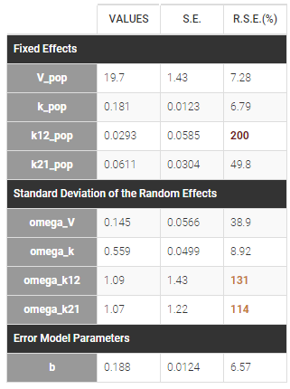
The parameters omega_k12 and omega_k21 have high standard errors, suggesting that the variability is difficult to estimate. The omega_k12 and omega_k21 values themselves are also high (100% inter-individual variability), suggesting that they may have been kept too high due to the simulated annealing.

• As a second step, we use the last estimates as new initial values (as shown here), and run SAEM again after disabling the simulated annealing option. On the plot showing the convergence of SAEM, we can see omega_V, omega_k12 and omega_k21 decreasing to very low values. The data is too sparse to correctly identify the inter-individual variability for V, k12 and k21. Thus, their random effects can be removed, but the random effect of k can be kept.

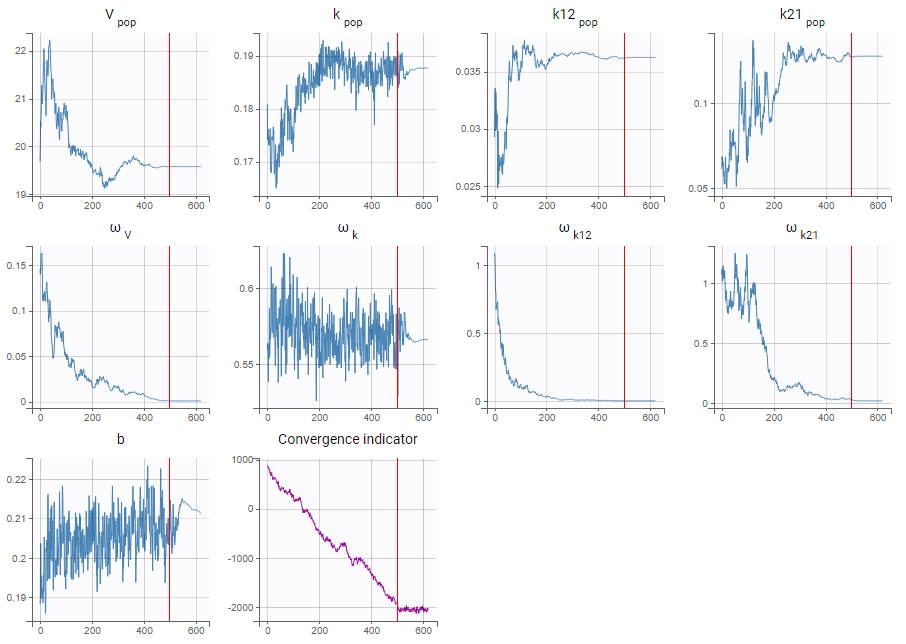
Note that because the omega_V, omega_k12 and omega_k21 parameters decrease without stabilizing, the convergence indicator does the same.