The estimation of the population parameters with SAEM includes a method of simulated annealing. It is possible to disable this option in the settings of SAEM. The option is enabled by default.
Purpose
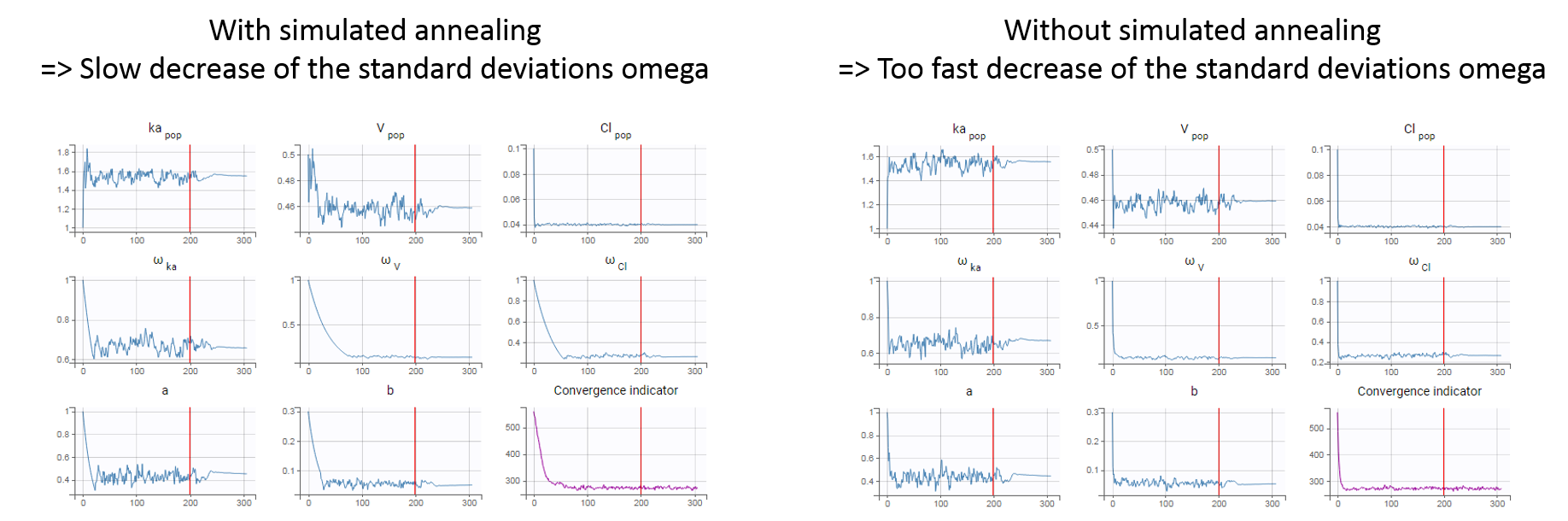
The simulated annealing option permits to keep the explored parameter space large for a longer time (compared to without simulated annealing). This allows to escape local maximums and improve the convergence towards the global maximum.
Calculations
In practice, the simulated annealing option constrains the variance of the random effects and the residual error parameters to decrease by maximum 5% (by default, the setting “Decreasing rate” can be changed) from one iteration to the next one. As a consequence, the variances decrease more slowly:
The size of the parameter space explored by SAEM depends on individual parameters sampled from their conditional distribution via Markov Chain Monte Carlo. If the standard deviation of the conditional distributions is large, the individual parameters sampled at iteration k can be quite far away from those at iteration (k-1), meaning a large exploration of the parameter space. The standard deviation of the conditional distribution depends on the standard deviation of the random effects (population parameters ‘omega’). Indeed, the conditional distribution is \(p(\psi_i|y_i;\hat{\theta})\) with \(\psi_i\) the individual parameters for individual \(i\), \(\hat{\theta}\) the estimated population parameters, and \(y_i\) the data (observations) for individual \(i\). The conditional distribution thus depends on the population parameters, and the larger the population parameters ‘omega’, the larger the standard deviation of the conditional distribution. That’s why we want to keep large ‘omega’ values during the first iterations.
Settings
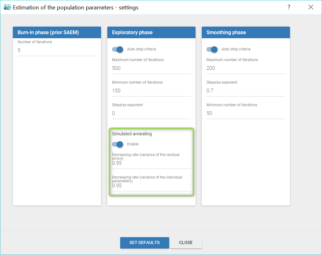
The simulated annealing option can be disabled or enabled in the “Population parameters” task settings. In addition, the settings allow to change the default decreasing rates for the standard deviations of the random effects and the residual errors.
Choosing to enable or disable the simulated annealing
As the simulated annealing option permits to more surely find the global maximum, it should be used during the first runs, when the initial values may be quite far from the final estimates.
On the other side, the simulated annealing option may keep the omega values artificially high, even after a large number of SAEM iterations. This may prevent the identification of parameters for which the variability is in fact zero and lead to NaN in the standard errors. So once good initial values have been found and there is no risk to fall in a local maximum, the simulated annealing option can be disabled. Below we show an example where removing the simulated annealing permits to identify parameters for which the inter-individual variability can be removed.
Example: identifying parameters with no variability
The dataset used in the tobramycin case study is quite sparse. In these conditions, we expect that estimating the inter-individual variability for all parameters will be difficult. In this case, the estimation can be done in two steps, as shown below for a two-compartments model on this dataset:
- First, we run SAEM with the simulated annealing option (default setting), which facilitates the convergence towards the global maximum. All four parameters V, k, k12 and k21 have random effects. The estimated parameters are shown below:
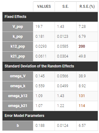
The parameters omega_k12 and omega_k21 have high standard errors, suggesting that the variability is difficult to estimate. The omega_k12 and omega_k21 values themselves are also high (100% inter-individual variability), suggesting that they may have been kept too high due to the simulated annealing.
- As a second step, we use the last estimates as new initial values (as shown here), and run SAEM again after disabling the simulated annealing option. On the plot showing the convergence of SAEM, we can see omega_V, omega_k12 and omega_k21 decreasing to very low values. The data is then too sparse to correctly identify the inter-individual variability for V, k12 and k21. Thus, their random effects can be removed, but the random effect of k can be kept.
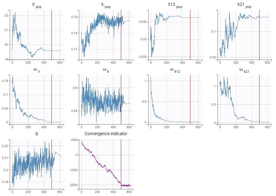
Note that because the omega_V, omega_k12 and omega_k21 parameters decrease without stabilizing, the convergence indicator does the same.