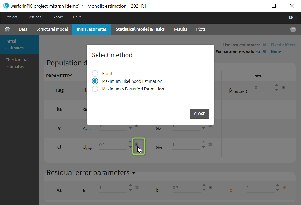
In the tab “Initial estimates”, clicking on the wheel icon next to a population parameters opens a window to choose among three estimation methods (see image below). “Maximum Likelihood Estimation” corresponds to the default method using SAEM, detailed on this page. “Maximum A Posteriori Estimation” corresponds to Bayesian estimation, and “Fixed” to a fixed parameter.
Bayesian estimation
Purpose
Bayesian estimation allows to take into account prior information in the estimation of parameters. It is called in Monolix Maximum A Posteriori estimation, and it corresponds to a penalized maximum likelihood estimation, based on a prior distribution defined for a parameter. The weight of the prior in the estimation is given by the standard deviation of the prior distribution.
Objectives: learn how to combine maximum likelihood estimation and Bayesian estimation of the population parameters.
Projects: theobayes1_project, theobayes2_project,
Introduction
The Bayesian approach considers the vector of population parameters \(\theta\) as a random vector with a prior distribution \(\pi_\theta\). We can then define the *posterior distribution* of \(\theta\):
\(\begin{aligned} p(\theta | y ) &= \frac{\pi_\theta( \theta )p(y | \theta )}{p(y)} \\ &= \frac{\pi_\theta( \theta ) \int p(y,\psi |\theta) \, d \psi}{p(y)} . \end{aligned} \)
We can estimate this conditional distribution and derive statistics (posterior mean, standard deviation, quantiles, etc.) and the so-called maximum a posteriori (MAP) estimate of \(\theta\):
\(\begin{aligned} \hat{\theta}^{\rm MAP} &=\text{arg~max}_{\theta} p(\theta | y ) \\ &=\text{arg~max}_{\theta} \left\{ {\cal LL}_y(\theta) + \log( \pi_\theta( \theta ) ) \right\} . \end{aligned} \)
The MAP estimate maximizes a penalized version of the observed likelihood. In other words, MAP estimation is the same as penalized maximum likelihood estimation. Suppose for instance that \(\theta\) is a scalar parameter and the prior is a normal distribution with mean \(\theta_0\) and variance \(\gamma^2\). Then, the MAP estimate is the solution of the following minimization problem:
\(\hat{\theta}^{\rm MAP} =\text{arg~min}_{\theta} \left\{ -2{\cal LL}_y(\theta) + \frac{1}{\gamma^2}(\theta – \theta_0)^2 \right\} .\)
This is a trade-off between the MLE which minimizes the deviance, \(-2{\cal LL}_y(\theta)\), and \(\theta_0\) which minimizes \((\theta – \theta_0)^2\). The weight given to the prior directly depends on the variance of the prior distribution: the smaller \(\gamma^2\) is, the closer to \(\theta_0\) the MAP is. In the limiting case, \(\gamma^2=0\); this means that \(\theta\) is fixed at \(\theta_0\) and no longer needs to be estimated. Both the Bayesian and frequentist approaches have their supporters and detractors. But rather than being dogmatic and following the same rule-book every time, we need to be pragmatic and ask the right methodological questions when confronted with a new problem.
All things considered, the problem comes down to knowing whether the data contains sufficient information to answer a given question, and whether some other information may be available to help answer it. This is the essence of the art of modeling: find the right compromise between the confidence we have in the data and our prior knowledge of the problem. Each problem is different and requires a specific approach. For instance, if all the patients in a clinical trial have essentially the same weight, it is pointless to estimate a relationship between weight and the model’s PK parameters using the trial data. A modeler would be better served trying to use prior information based on physiological knowledge rather than just some statistical criterion.
Generally speaking, if prior information is available it should be used, on the condition of course that it is relevant. For continuous data for example, what does putting a prior on the residual error model’s parameters mean in reality? A reasoned statistical approach consists of including prior information only for certain parameters (those for which we have real prior information) and having confidence in the data for the others. Monolix allows this hybrid approach which reconciles the Bayesian and frequentist approaches. A given parameter can be
- a fixed constant if we have absolute confidence in its value or the data does not allow it to be estimated, essentially due to lack of identifiability.
- estimated by maximum likelihood, either because we have great confidence in the data or no information on the parameter.
- estimated by introducing a prior and calculating the MAP estimate or estimating the posterior distribution.
Computing the Maximum a posteriori (MAP) estimate
- demo project: theobayes1_project (data = ‘theophylline_data.txt’ , model = ‘lib:oral1_1cpt_kaVCl.txt’)
We want to introduce a prior distribution for \(ka_{\rm pop}\) in this example. Click on the option button

and select Maximum A Poteriori Estimation

We propose a typical value, here 2 and standard deviation 0.1 for \(ka_{\rm pop}\) and to compute the MAP estimate for \(ka_{\rm pop}\). The parameter is then colored in purple.

Starting from the 2021 version, it is possible to select maximum a posteriori estimation also for the omega parameters (standard deviations of the random effects). In this case, an inverse Wishart is set as a prior distribution for the omega matrix.
The following distributions for the priors are used:
- typical value (*_pop): the distribution of the prior is the same as the distribution of the parameter. For instance, if ka has been set with a lognormal distribution in the “Statistical model & Tasks” tab, a lognormal distribution is also used for the prior on ka_pop. When a lognormal distribution is used, setting sd=0.1 roughtly corresponds to 10% uncertainty in the provided prior value for ka_pop.
- covariate effects (beta_*): a normal distribution is used, to allow betas to be either positive or negative.
- standard deviations (omega_*) [starting version 2021]: an inverse Wishart distribution is used. Inverse Wisharts are common prior distributions for variance-covariance matrices as they allow to fulfill the positive-definite matrix requirement. The weight of the prior in the estimation is based on the number of degrees of freedom (df) of the inverse Wishart, instead of a standard deviation. More degrees of freedom correspond to a higher constrain of the prior in the omega estimation. In Monolix, each omega parameter is handled as a 1×1 matrix with its own degree of freedom, independently from the other omegas. The univariate inverse Wishart \( W^{-1}(df, (df+2)\omega_{typ}) \) simplifies to an inverse gamma distribution with shape parameter \(\alpha=df/2 \) and scale parameter \(\beta=\omega_{typ}*(df+2)/2\). The coefficient of variation is thus \(CV=\frac{1}{\sqrt{\frac{df}{2}-2}}\). To obtain a 20% uncertainty on omega (CV=0.2), the user can set df=50.
- correlations: it is currently not possible to set a prior on the correlation parameters
It is common to set the initial value of the parameter to be the same as the typical value of the prior. Note that the default value for the typical value of the prior is set to the initial value of the parameter. However, if the initial value of the parameter is modified afterwards, the typical value of the prior is not updated automatically.
Fixing the value of a parameter
Population parameters can be fixed to their initial values, in this case they are not estimated. It is possible to fix one, several or all population parameters, among the fixed effects, standard deviations of random effects, and error model parameters. In Monolix2021, it is also possible to fix correlation parameters.
To fix a population parameter, click on the wheel next to the parameter in the tab “Initial estimates” and select “Fixed”, like on the image below:
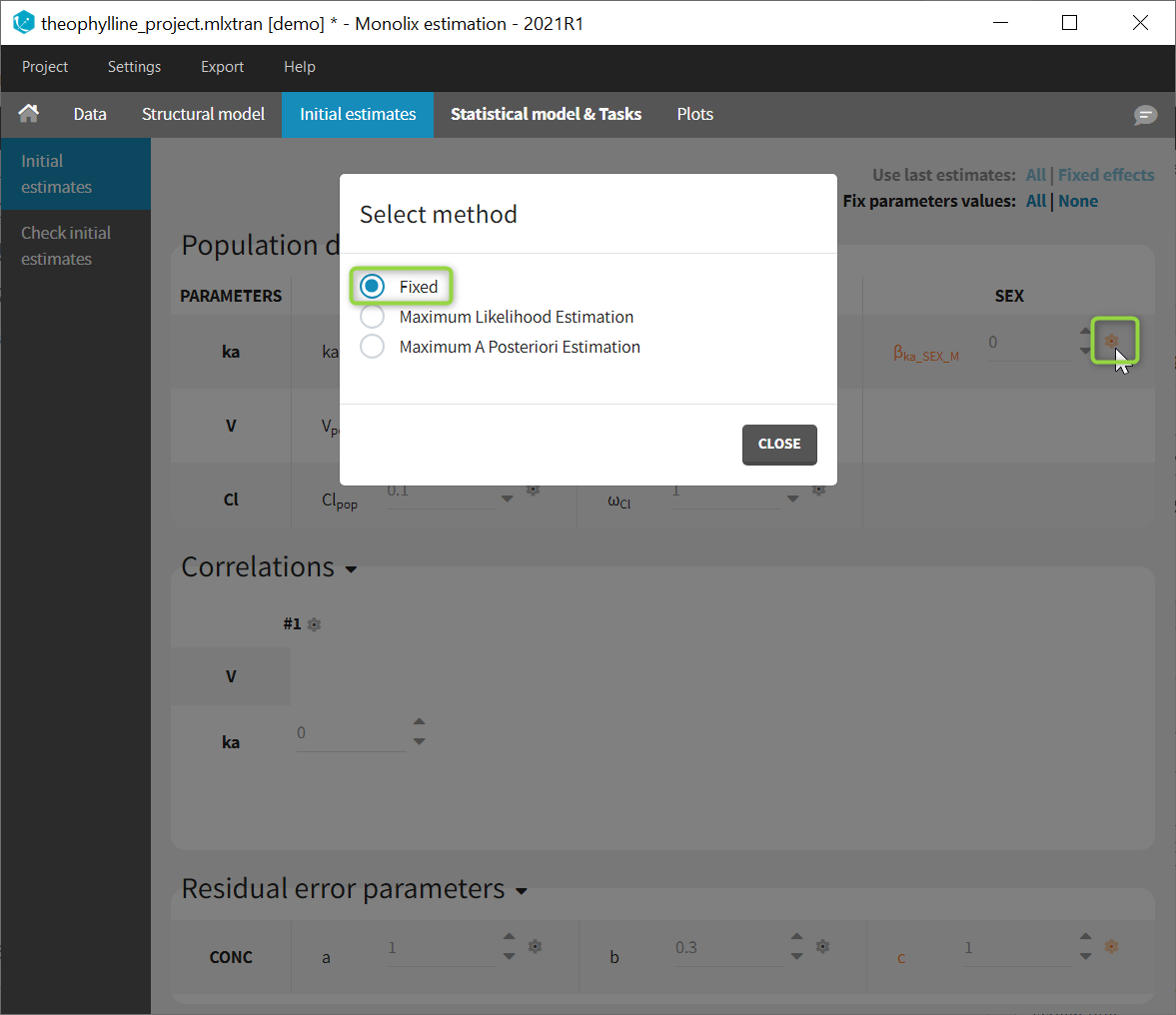
Fixed parameters appear on this tab in red. In Monolix2021, they are also colored in red in the subtab “Check initial estimates”.
- theobayes2_project (data = ‘theophylline_data.txt’ , model = ‘lib:oral1_1cpt_kaVCl.txt’)
We can combine different strategies for the population parameters: Bayesian estimation for \(ka_{\rm pop}\), fixed value for \(V_{\rm pop}\) and maximum likelihood estimation for \(Cl_{\rm pop}\), for instance.

Remark:
- The parameter \(V_{\rm pop}\) is fixed and then colored in red.
- \(V_{\rm pop}\) is not estimated (it’s s.e. is not computed) but the standard deviation \(\omega_{V}\) is estimated as usual.