- Introduction
- Formatting of count data in the MonolixSuite
- Count data with constant distribution over time
- Count data with time varying distribution
Objectives: learn how to implement a model for count data.
Projects: count1a_project, count1a_project, count1a_project, count2_project
Introduction
Longitudinal count data is a special type of longitudinal data that can take only nonnegative integer values {0, 1, 2, …} that come from counting something, e.g., the number of seizures, hemorrhages or lesions in each given time period . In this context, data from individual j is the sequence \(y_i=(y_{ij},1\leq j \leq n_i)\) where \(y_{ij}\) is the number of events observed in the jth time interval \(I_{ij}\).
Count data models can also be used for modeling other types of data such as the number of trials required for completing a given task or the number of successes (or failures) during some exercise. Here, \(y_{ij}\) is either the number of trials or successes (or failures) for subject i at time \(t_{ij}\). For any of these data types we will then model \(y_i=(y_{ij},1 \leq j \leq n_i)\) as a sequence of random variables that take their values in {0, 1, 2, …}. If we assume that they are independent, then the model is completely defined by the probability mass functions \(\mathbb{P}(y_{ij}=k)\) for \(k \geq 0\) and \(1 \leq j \leq n_i\). Here, we will only consider parametric distributions for count data.
Formatting of count data in the MonolixSuite
Count data can only take non-negative integer values that come from counting something, e.g., the number of trials required for completing a given task. The task can for instance be repeated several times and the individual’s performance followed. In the following data set:
ID TIME Y
1 0 10
1 24 6
1 48 5
1 72 2
10 trials are necessary the first day (t=0), 6 the second day (t=24), etc. Count data can also represent the number of events happening in regularly spaced intervals, e.g the number of seizures every week. If the time intervals are not regular, the data may be considered as repeated time-to-event interval censored, or the interval length can be given as regressor to be used to define the probability distribution in the model.
One can see the epilepsy attacks data set for a more practical example.
Modling count data in the MonolixSuite
Link to the detailed description of the library of count models integrated within Monolix.
Count data with constant distribution over time
- count1a_project (data = ‘count1_data.txt’, model = ‘count_library/poisson_mlxt.txt’)
A Poisson model is used for fitting the data:
[LONGITUDINAL]
input = lambda

DEFINITION:
Y = {type = count,  log(P(Y=k)) = -lambda + k*log(lambda) - factln(k) }

OUTPUT:
output = Y
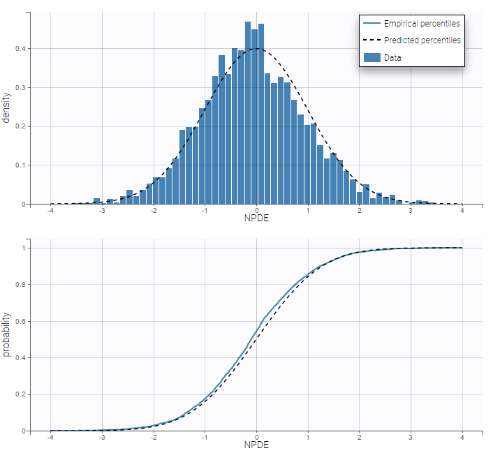
Residuals for noncontinuous data reduce to NPDEs. We can compare the empirical distribution of the NPDEs with the distribution of a standardized normal distribution either with the pdf (top) or the cdf (bottom):
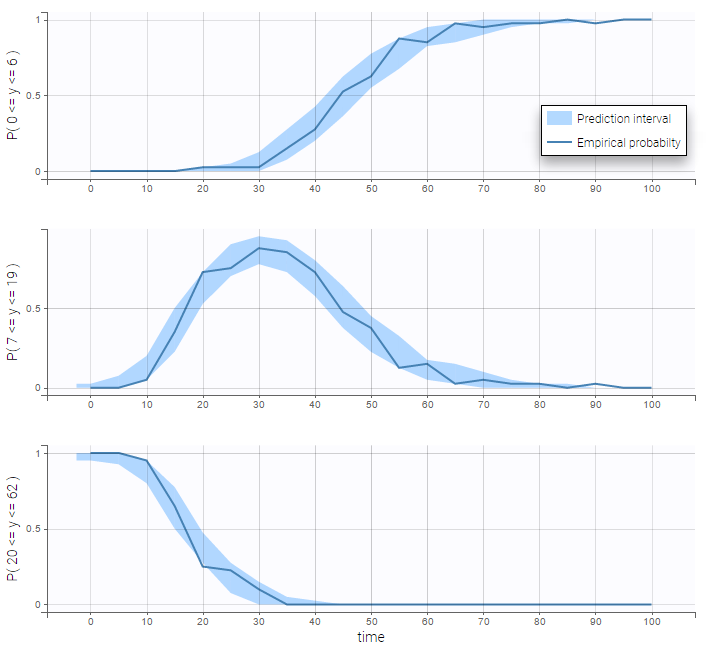
VPCs for count data compare the observed and predicted frequencies of the categorized data over time:
- count1b_project (data = ‘count1_data.txt’, model = ‘count_library/poissonMixture_mlxt.txt’)
A mixture of two Poisson distributions is used to fit the same data. For that, we define the probability of k occurrences as the weigthed sum of two Poisson distributions with two expected numbers of occurrences lambda1 and lambda2. The structural model file writes
[LONGITUDINAL]
input = {lambda1, alpha, mp}

EQUATION:
lambda2 = (1+alpha)*lambda1

DEFINITION:
Y = { type = count,
       P(Y=k) = mp*exp(-lambda1 + k*log(lambda1) - factln(k)) + (1-mp)*exp(-lambda2 + k*log(lambda2) - factln(k))
}

OUTPUT:
output = Y
Thus, the parameter alpha has to be strictly positive to ensure different expected number of occurrences in the two poisson distributions and mp has to be in [0, 1] to ensure the probability is correctly defined. Thus those parameters should be defined with lognormal and probitnormal distribution respectively as shown on the following figure.

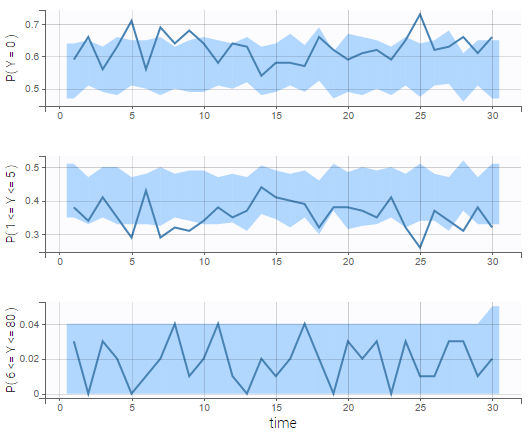
We see on the VPC below that the data set is well modeled using this mixture of Poisson distributions.
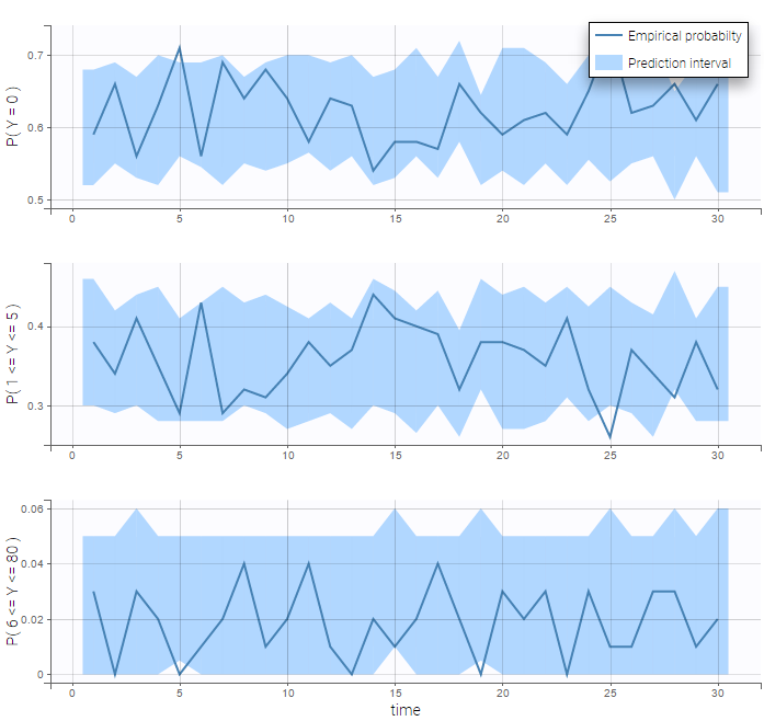
In addition, we can compute the prediction distribution of the modalities as on the following figure
Count data with time varying distribution
- count2_project (data = ‘count2_data.txt’, model = ‘count_library/poissonTimeVarying_mlxt.txt’)
The distribution of the data changes with time in this example:
We then use a Poisson distribution with a time varying intensity:
[LONGITUDINAL]
input =  {a,b}

EQUATION:
lambda= a*exp(-b*t)

DEFINITION:
y = {type=count, P(y=k)=exp(-lambda)*(lambda^k)/factorial(k)}

OUTPUT:
output = y
This model seems to fit the data very well: