- Model with continuous covariates
- Model with categorical covariates
- Transforming categorical covariates
- The same covariate effect for several parameters
- Complex parameter covariate relationships (such as Michaelis-Menten or Hill dependencies, time-dependent covariates, or covariate-dependent standard deviations of random effects)
Objectives: learn how to implement a model for continuous and/or categorical covariates.
Projects: warfarin_covariate1_project, warfarin_covariate2_project, warfarin_covariate3_project, phenobarbital_project
Model with continuous covariates
- warfarin_covariate1_project (data = ‘warfarin_data.txt’, model = ‘lib:oral1_1cpt_TlagkaVCl.txt’)
The warfarin data contains 2 individual covariates: weight which is a continuous covariate and sex which is a categorical covariate with 2 categories (1=Male, 0=Female). We can ignore these columns if are sure not to use them, or declare them using respectively the reserved keywords CONTINUOUS COVARIATE and CATEGORICAL COVARIATE to define continuous and categorical covariate.
Even if these 2 covariates are now available, we can choose to define a model without any covariate by not clicking on any check box in the covariate model.
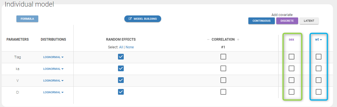
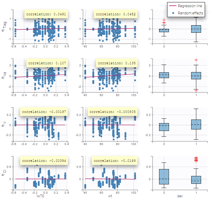
Here, an unchecked box in the line of the parameter V and the column of the covariate wt means that there is no relationship between weight and volume in the model. A diagnosis plot Individual parameters vs covariates is generated which displays possible relationships between covariates and individual parameters (even if these covariates are not used in the model):
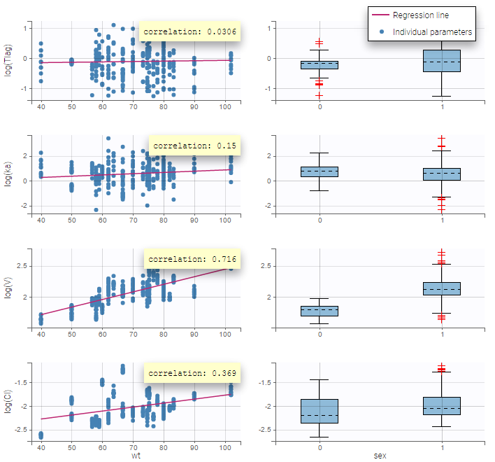
On the figure, we can see a strong correlation between the volume V and both the weight wt and the sex. One can also see a correlation between the clearance and the weight wt. Therefore, the next step is to add some covariate to our model.
- warfarin_covariate2_project (data = ‘warfarin_data.txt’, model = ‘lib:oral1_1cpt_TlagkaVCl.txt’)
We decide to use the weight in this project in order to explain part of the variability of \(V_i\) and \(Cl_i\). We will implement the following model for these two parameters:
$$\log(V_i) = \log(V_{\rm pop}) + \beta_V \log(w_i/70) + \eta_{V,i} ~~\text{and}~~\log(Cl_i) = \log(Cl_{\rm pop}) + \beta_{Cl} \log(w_i/70) + \eta_{Cl,i}$$
which means that population parameters of the PK parameters are defined for a typical individual of the population with weight = 70kg.
More details about the model
The model for \(V_{i}\) and \(Cl_{i}\) can be equivalently written as follows:
$$ V_i = V_{\rm pop} ( w_i/70 )^{\beta_V} e^{ \eta_{V,i} } ~~\text{and}~~ Cl_i = Cl_{\rm pop} ( w_i/70 )^{\beta_{Cl}} e^{ \eta_{Cl,i} }$$
The individual predicted values for \(V_i\) and \(Cl_i\) are therefore
$$\bar{V}_i = V_{\rm pop} \left( w_i/70 \right)^{\beta_V} ~~\text{and}~~ \bar{Cl}_i = Cl_{\rm pop} \left( w_i/70 \right)^{\beta_{Cl}} $$
and the statistical model describes how \(V_i\) and \(Cl_i\) are distributed around these predicted values:
$$ \log(V_i) \sim {\cal N}( \log(\bar{V}_i) , \omega^2_V) ~~\text{and}~~\log(Cl_i) \sim {\cal N}( \log(\bar{Cl}_i) , \omega^2_{Cl}) $$
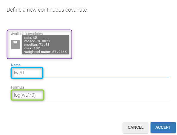
Here, \(\log(V_i)\) and \(\log(Cl_i)\) are linear functions of \(\log(w_i/70)\): we then need to transform first the original covariate \(w_i\) into \(\log(w_i/70)\) by clicking on the button CONTINUOUS next to ADD COVARIATE (blue button). Then, the following pop up arises
You have to
- define the name of the covariate you want to add (the blue frame).
- define the associated equation (the green frame).
- click on the ACCEPT button
Remarks
- You can define any formula for your covariate as long as you use mathematical functions available in the Mlxtran language.
- You can use any covariate available in the list of covariates proposed in the window. Thus, if you have a Height and Weight as covariates, you can directly compute the Body Mass Index.
- If you go over a covariate with your mouse, all the information (min, mean, median, max and weighted mean) are displayed as a tooltip. The weighted mean is defined as \[ \text{weighted mean} (cov) = \exp \Big( \sum_i \frac{\text{nbObs}_i }{\text{nbObs}} \log(cov_i) \Big)\] where \(\text{nbObs}_i\) is the number of observation for the \(i^{th}\) individual and \(\text{nbObs}\) is the total number of observations.
- If you click on the covariate name, it will be written in the formula.
- You can use this formula box to replace missing continuous covariate values by an imputed value. This is explained in the feature of the week #141 below. For example, if your continuous covariate takes only positive values, you can use a negative value for the missing values in your dataset, for example -99, and enter the following formula: max(COV,0) + min(COV,0)/COV*ImputedValue with the desired ImputedValue (COV is thAse name of your covariate).
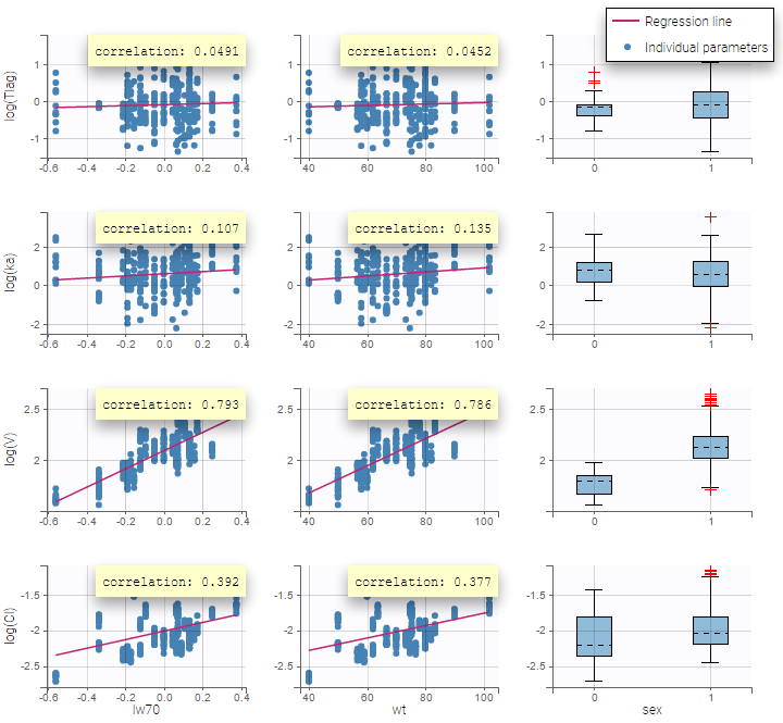
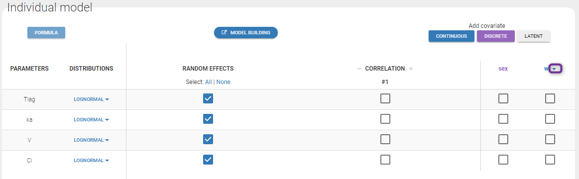
We then define a new covariate model, where \(\log(V_i)\) and \(\log(Cl_i)\) are linear functions of the transformed weight \(lw70_i\) as shown on the following figure:

Notice that by clicking on the button FORMULA, you have the display of all the individual model equations. Coefficients \(\beta_{V}\) and \(\beta_{Cl}\) are now estimated with their s.e. and the p-values of the Wald tests are derived to test if these coefficients are different from 0.
Again, a diagnosis plot Individual parameters vs covariates is generated which displays possible relationships between covariates and individual parameters (even if these covariates are not used in the model) as one can see on the figure below on the left. However, as there are covariates on the model, what is interesting is to see if there still are correlation between the random effects and the covariates as one can see on the figure below on the right.
 |
 |
|---|
Note: To make it automatically, starting from the 2019 version, there is an arrow next (in purple in the next figure) to the continuous covariate from the data set and propose to add a log transformed covariate centered by the weighted mean.
Model with categorical covariates
- warfarin_covariate3_project (data = ‘warfarin_data.txt’, model = ‘lib:oral1_1cpt_TlagkaVCl.txt’)
We use sex instead of weight in this project, assuming different population values of volume and clearance for males and females. More precisely, we consider the following model for \(V_i\) and \(Cl_i\):
$$\log(V_i) = \log(V_{\rm pop}) + \beta_V 1_{sex_i=F} + \eta_{V,i}~~\text{and}~~\log(Cl_i) = \log(Cl_{\rm pop}) + \beta_{Cl} 1_{sex_i=F} + \eta_{Cl,i}$$
where \(1_{sex_i=F} =1\) if individual i is a female and 0 otherwise. Then, \(V_{\rm pop}\) and \(Cl_{\rm pop}\) are the population volume and clearance for males while \(V_{\rm pop}, e^{\beta_V}\) and \(Cl_{\rm pop} e^{\beta_{Cl}}\) are the population volume and clearance for females. By clicking on the purple button DISCRETE, the following window pops up

You have to
- define the name of the covariate you want to add (the blue frame).
- define the associated categories (the green frame).
- click on the ALLOCATE button to define all the categories.
Then, you can
- define the name of the categories (the blue frame).
- define the reference category (the green frame).
- click on ACCEPT
Then, define the covariate model in the main GUI:

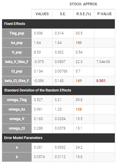
Estimated population parameters, including the coefficients \(\beta_V\) and \(\beta_{Cl}\) are displayed with the results:
 We can display the probability distribution functions of the 4 PK parameters using the
 Individual parameter graphic:
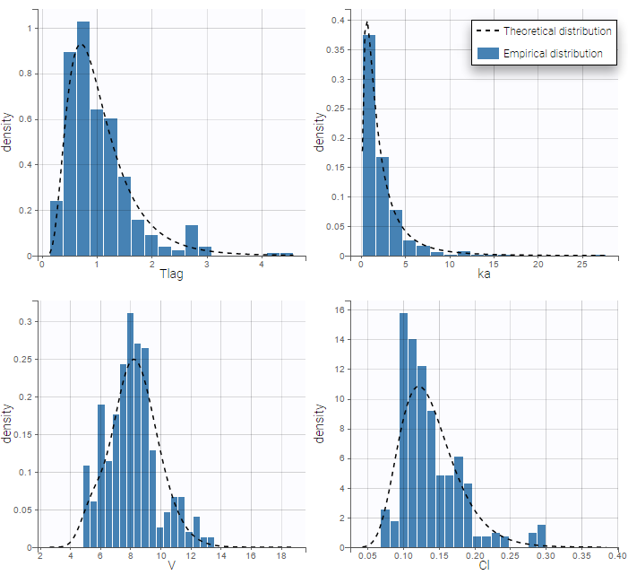
Notice that for the volume and the clearance, the theoretical curve is is not the PDF of a lognormal distribution, due to the impact of the covariate sex.
Calculating the typical value for each category
Cl_pop represents the typical value for the reference category (in the example above SEX=0). The typical value for the other categories can be calculated based on the estimated beta parameters:
- normal distribution: \( Cl_{SEX=1} = Cl_{pop} + beta\_Cl\_SEX\_1 \)
- lognormal distribution: \( Cl_{SEX=1} = Cl_{pop} \times e^{beta\_Cl\_SEX\_1 } \)
- logit distribution: \( F_{SEX=1} = \frac{1}{1+ e^{-\left( \log \left(\frac{F_{pop}}{1-F_{pop}} \right) + beta\_F\_SEX\_1 \right) }} \)
Transforming categorical covariates
- phenobarbital_project (data = ‘phenobarbital_data.txt’, model = ‘lib:bolus_1cpt_Vk.txt’)
The phenobarbital data contains 2 covariates: the weight and the APGAR score which is considered as a categorical covariate. Instead of using the 10 original levels of the APGAR score, we will transform this categorical covariate and create 3 categories: Low = {1,2,3}, Medium = {4, 5, 6, 7} and High={8,9,10}.

If we assume, for instance that the volume is related to the APGAR score, then \(\beta_{V,Low}\) and \(\beta_{V,High}\) are estimated (assuming that Medium is the reference level).
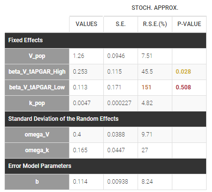
In that case, one can see that both p-values concerning the transformed APGAR covariate are over .05.
The same covariate effect for several parameters
Adding a covariate effect on a parameter in the Individual Model section of the Statistical Model and Tasks tab, creates automatically a corresponding beta parameter (population parameter) that describes the strength of the effect. For example, adding weight WT on a parameter volume V1 creates beta_V1_WT. If you add the same covariate effect on two different parameters, eg. V1 and V2, then Monolix will create two corresponding parameters: beta_V1_WT and beta_V2_WT.
If you need to add the same covariate effect for several parameters, eg. have only one parameter betaWT for both V1 and V2 in the example above, then this covariate effect has to be implemented in the structural model directly. It requires:
-
Reading weight WT from the dataset, so the columnt WT in the dataset has to be tagged as a regressor (not covariate)
-
Defining in the model new volumes with the covariate effect (sample code below, based on a two-compartment model from the PK library)[LONGITUDINAL]input = {WT, betaWT, ka, Cl, V1, Q2, V2}WT = {use=regressor}PK:; Effect of WT on V1, V2V1_withWT = V1*exp(betaWT*WT)V2_withWT = V2*exp(betaWT*WT); Parameter transformationsV = V1_withWTk12 = Q2/V1_withWTk21 = Q2/V2_withWT; PK model definitionCc = pkmodel(ka, V, Cl, k12, k21)OUTPUT:output = {Cc}
-
In the Individual model in the GUI, set normal distribution for “betaWT” – to allow positive and negative values, and remove random effects from it – they are already included in the parameters V1, V2.