To start a new Monolix project, you need to define a dataset by loading a file in the Data tab, and load a model in the structural model tab. The project can be saved only after defining the data and the model.
Supported file types: Supported file types include .txt, .csv, and .tsv files. Starting with version 2024, additional Excel and SAS file types are supported: .xls, .xlsx, .sas2bdat, and .xpt files in addition to .txt, .csv, and .tsv files.
The data set format expected in the Data tab is the same as for the entire MonolixSuite, to allow smooth transitions between applications. The columns available in this format and example datasets are detailed on this page. Briefly:
- Each line corresponds to one individual and one time point
- Each line can include a single measurement (also called observation), or a dose amount (or both a measurement and a dose amount)
- Dosing information should be indicated for each individual, even if it is identical for all.
Your dataset may not be originally in this format, and you may want to add information on dose amounts, limits of quantification, units, or filter part of the dataset. To do so, you should proceed in this order:
- Formatting: If needed, format your data first by loading the dataset in the Data Formatting tab. Briefly, it allows to:
- to deal with several header lines
- merge several observation columns into one
- add censoring information based on tags in the observation column
- add treatment information manually or from external sources
- add more columns based on another file
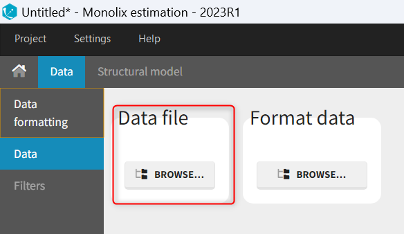
- Loading a new data set: If the data is already in the right format, load it directly in the Data tab (otherwise use the formatted dataset created by data formatting).
- Observation types: Specify if the observation is of type continuous, count/categorical or event.
- Labeling: label the columns not recognized automatically to indicate their type and click on ACCEPT.
- Filtering: If needed, filter your dataset to use only part of it in the Filters tab
- Explore: The interpreted dataset is displayed in Data, and Plots and covariate statistics are generated.
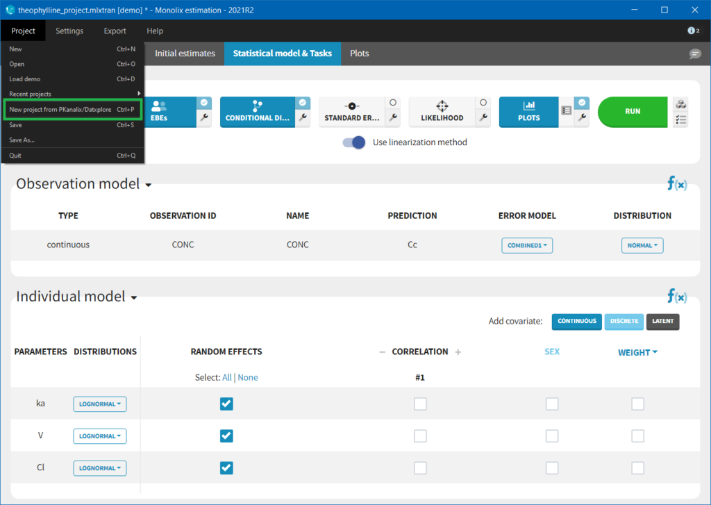
If you have already defined a dataset in Datxplore or in PKanalix, you can skip all those steps in Monolix and create a new project by importing a project from Datxplore or PKanalix.
Loading a new data set
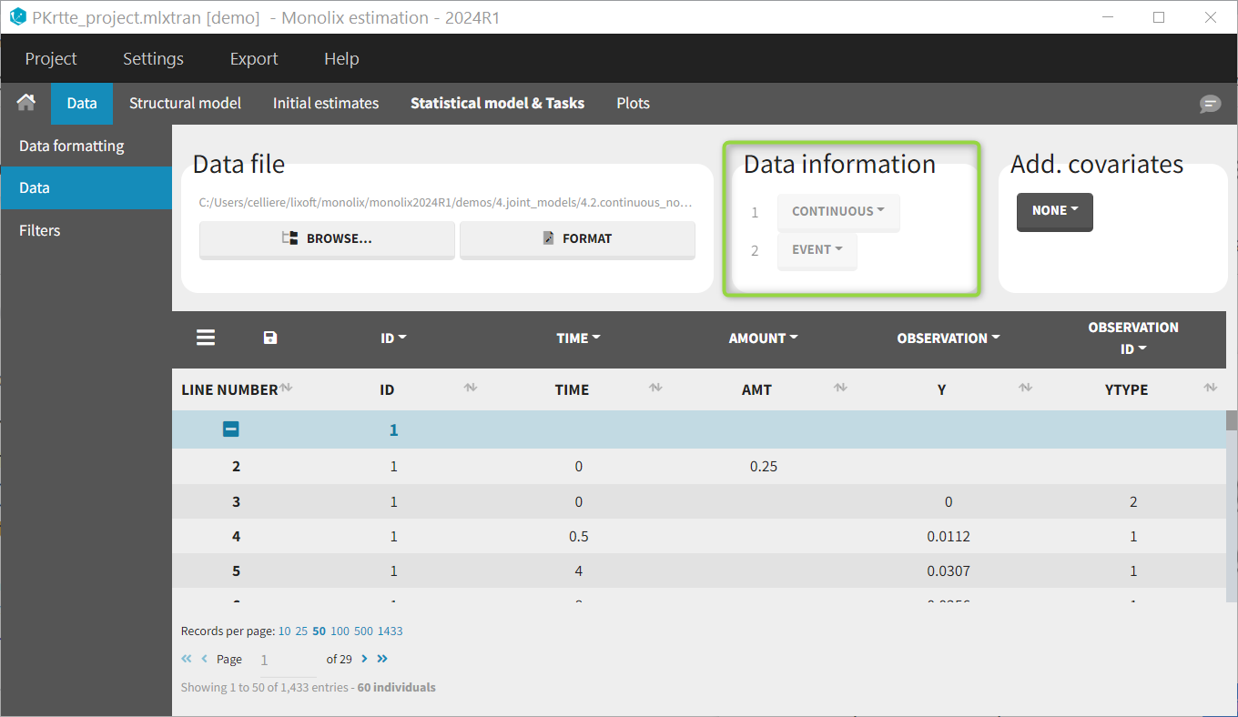
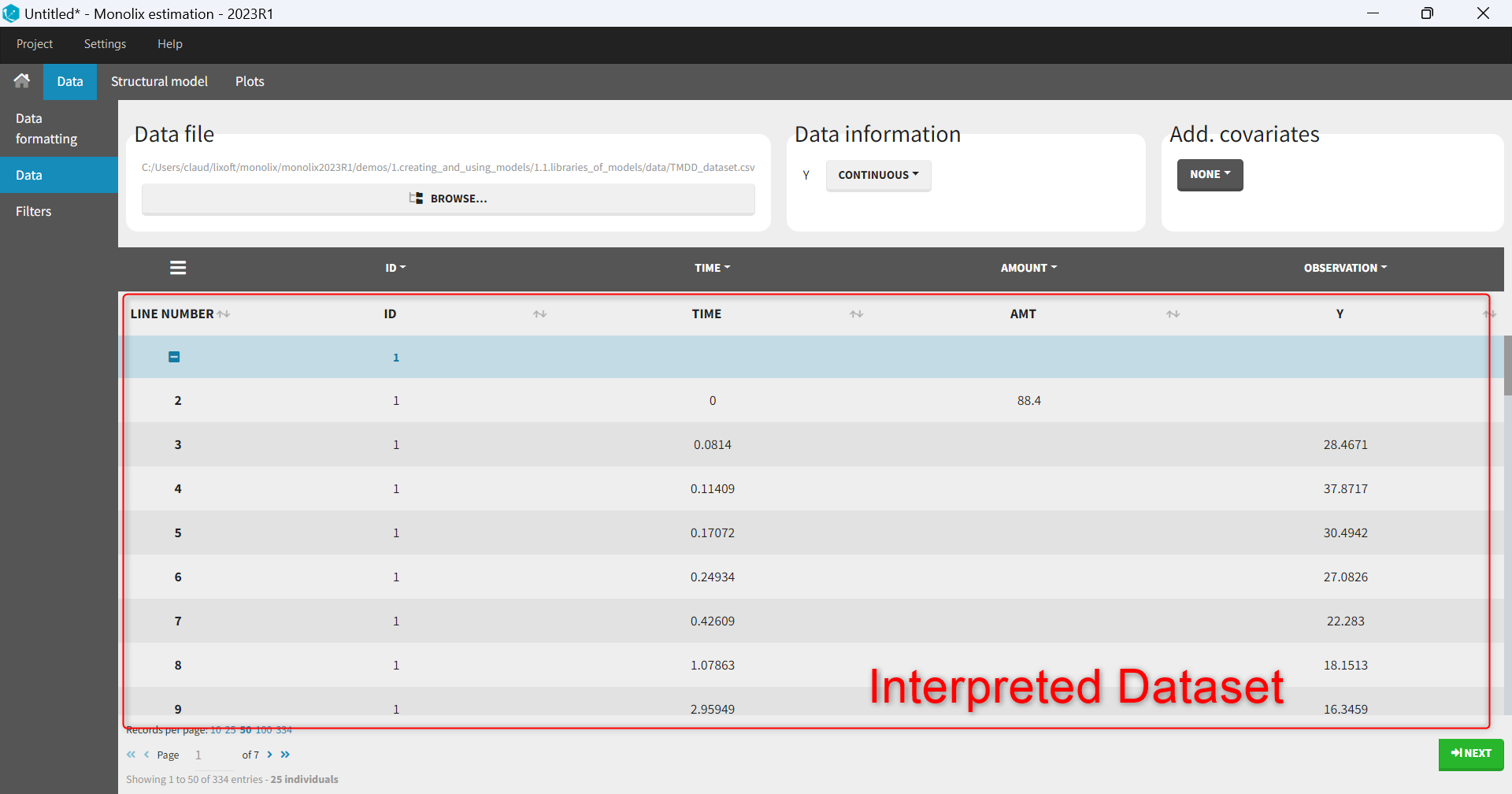
To load a new data set, you have to go to “Browse” your data set (green frame), tag all the columns (purple frame), define the observation types in Data Information (blue frame), and click on the blue button ACCEPT as on the following. If the dataset does not follow a formatting rule, the dataset will not be accepted, but errors will guide you to find what is missing and could be added by data formatting.
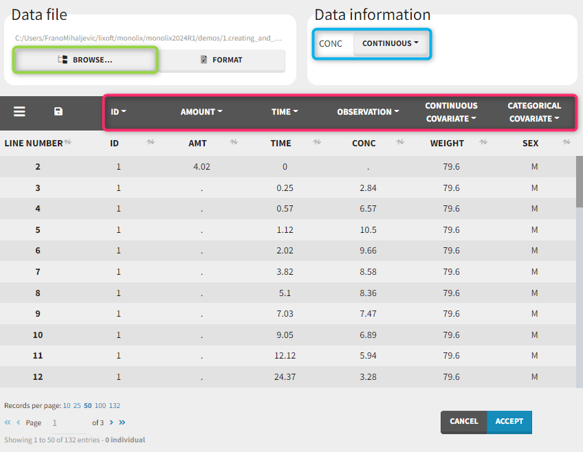
Observation types
There are three types of observations:
- continuous: The observation is continuous and can take any value within a range. For example, a concentration is a continuous observation.
- count/categorical: The observation values can take values only in a finite categorical space. For example, the observation can be a categorical observation (an effect can be observed as “low”, “medium”, or “high”) or a count observation over a defined time (the number of epileptic crisis in a week).
- event: The observation is an event, for example the time of death.
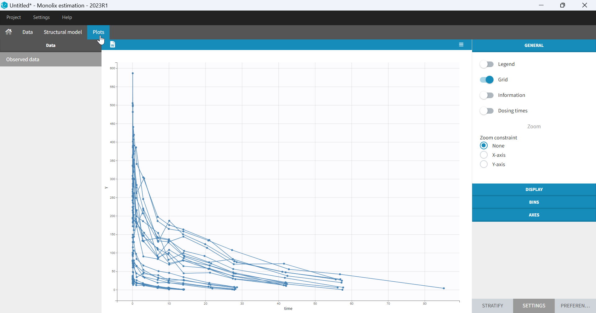
For each OBSERVATION ID, the type of observations must be specified by the user in the interface. Depending on the choice, the data will be displayed in the Observed Data plot in different ways (e.g spaghetti plot for continuous data and Kaplan-Meier plot for event data). The mapping of model outputs and observations from the dataset will also take into account the data type (e.g a model outptu of type “event” can only be mapped to an observation that is also an “event”). Once a model has been selected, the choice of the data types are locked (because they are enforced by the model output type).
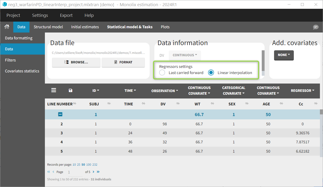
Regressor settings
If columns have been tagged as REGRESSORS, the interpolation method for the regressors can be chosen. In the dataset, regressors are defined only for a finite number of time points. In between those time points, the regressor values can be interpolated in two different ways:
- last carried forward: if we have defined in the dataset two times for each individual with \(reg_A\) at time \(t_A\) and \(reg_B\) at time \(t_B\)
- for \(t\le t_A\), \(reg(t)=reg_A\) [first defined value is used]
- for \(t_A\le t<t_B\), \(reg(t)=reg_A\) [previous value is used]
- for \(t>t_B\), \(reg(t)=reg_B\) [previous value is used]
- linear interpolation: the interpolation is:
- for \(t\le t_A\), \(reg(t)=reg_A\) [first defined value is used]
- for \(t_A\le t<t_B\), \(reg(t)=reg_A+(t-t_A)\frac{(reg_B-reg_A)}{(t_B-t_A)}\) [linear interpolation is used]
- for \(t>t_B\), \(reg(t)=reg_B\) [previous value is used]
The interpolation is used to obtain the regressor value at times not defined in the dataset. This is necessary to integrate ODE-based models (which are using an internal adaptative time step), or obtain prediction on a fine grid for the plots (e.g in the Individuals fits) for instance.
When some dataset lines have a missing regressor value (dot “.”), the same interpolation method is used.
Labeling (column tagging)
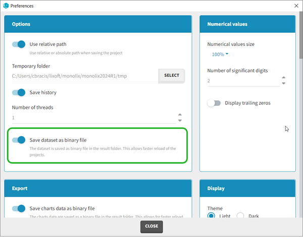
The column type suggested automatically by Monolix based on the headers in the data can be customized in the preferences. By clicking on Settings>Preferences, the following windows pops up.
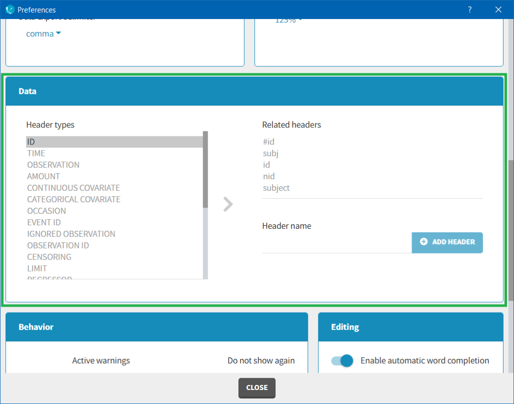
In the DATA frame, you can add or remove preferences for each column.
To remove a preference, double-click on the preference you would like to remove. A confirmation window will be proposed.
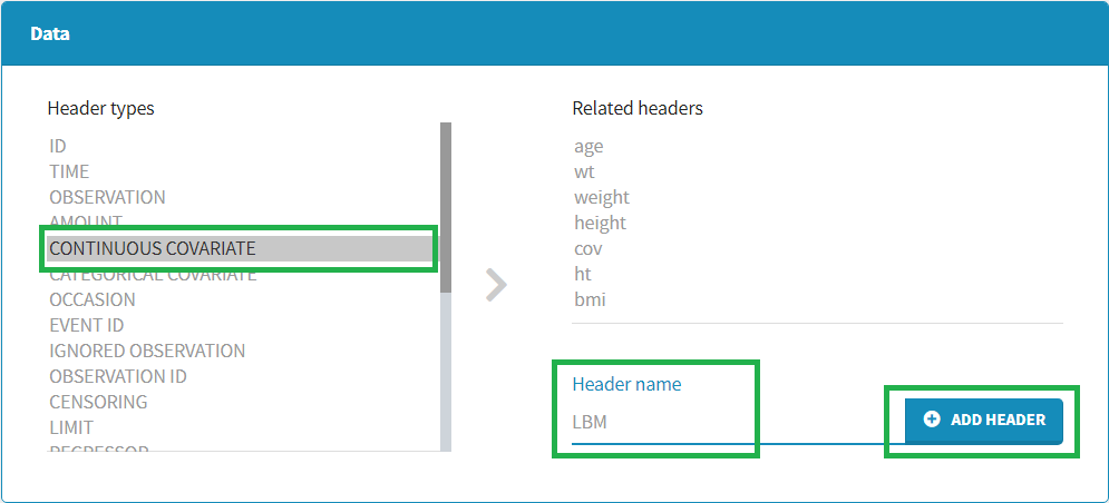
To add a preference, click on the header type you consider, add a name in the header name and click on “ADD HEADER” as on the following figure.
Notice that all the preferences are shared between Monolix, Datxplore, and PKanalix.
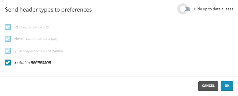
Starting from the version 2024, it is also possible to update the preferences with the columns tagged in the opened project, by clicking on the icon in the top left corner of the table:
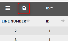
Clicking on the icon will open a modal with the option to choose which of the tagged headers a user wants to add to preferences:
Dataset load times
Starting with the 2024 version, it is possible to improve the project load times, especially for projects with large datasets, but saving the data as a binary file. This option is available in Settings>Preferences and will save a copy of the data file in binary format in the results folder. When reloading a project, the dataset will be read from the binary file, which will be faster. If the original dataset file has been modified (compared to the binary), a warning message will appear, the binary dataset will not be used and the original dataset fiel will be loaded instead.
Resulting plots and tables to explore the data
Once the dataset is accepted:
- Plots are automatically generated based on the interpreted dataset to help you proceed with a first data exploration before running any task.
- The interpreted dataset appears in Data tab, which incorporates all changes after formatting and filtering.
- Covariate Statistics appear in a section of the data tab.
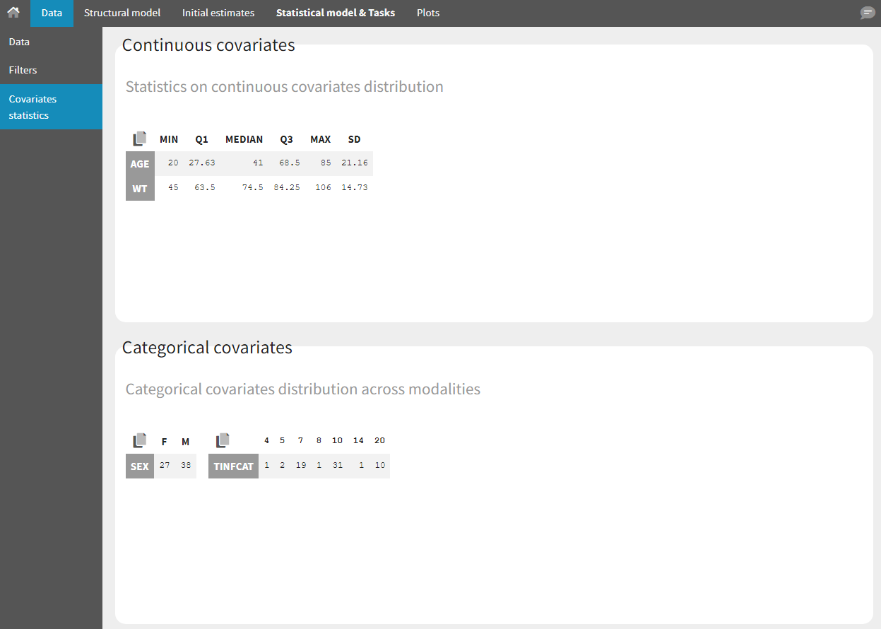
All the covariates (if any) are displayed and a summary of the statistics is proposed. For continuous covariates, minimum, median and maximum values are proposed along with the first and third quartile, and the standard deviation. For categorical covariates, all the modalities are displayed along with the number of each. Note the “Copy table” button that allows to copy the table in Word and Excel. The format and the display of the table will be preserved.
Importing a project from Datxplore or PKanalix
It is possible to import a project from Datxplore or PKanalix. For that, go to Project>New project for Datxplore/PKanalix (as in the green box of the following figure). In that case, a new project will be created and all the DATA frame will already be filled by the information from the Datxplore or PKanalix project.