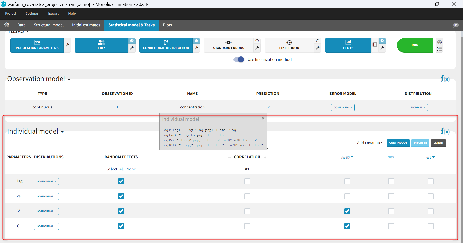
What is the individual model and where is it defined in Monolix?
The population approach considers that parameters of the structural model can have a different value for each individual, and the way these values are distributed over individuals and impacted by covariate values is defined in the individual model. The individual model is defined in the lower part of the statistical model tab. This model includes
- distributions for the individual parameters
- which parameters have inter-individual variability (random effects)
- correlation structure of the random effects
- covariate effects on the individual parameters
Theory for the individual model
A model for observations depends on a vector of individual parameters \(\psi_i\). As we want to work with a population approach, we now suppose that \(\psi_i\) comes from some probability distribution \(p_{{\psi_i}}\).
In this section, we are interested in the implementation of individual parameter distributions \((p_{{\psi_i}}, 1\leq i \leq N)\). Generally speaking, we assume that individuals are independent. This means that in the following analysis, it is sufficient to take a closer look at the distribution \(p_{{\psi_i}}\) of a unique individual i. The distribution \(p_{{\psi_i}}\) plays a fundamental role since it describes the inter-individual variability of the individual parameter \(\psi_i\). In Monolix, we consider that some transformation of the individual parameters is normally distributed and is a linear function of the covariates:
\(h(\psi_i) = h(\psi_{\rm pop})+ \beta \cdot ({c}_i – {c}_{\rm pop}) + \eta_i \,, \quad \eta_i \sim {\cal N}(0,\Omega).\)
This model gives a clear and easily interpreted decomposition of the variability of \(h(\psi_i)\) around \(h(\psi_{\rm pop})\), i.e., of \(\psi_i\) around \(\psi_{\rm pop}\):
The component \(\beta \cdot ({c}_i – {c}_{\rm pop})\) describes part of this variability by way of covariates \({c}_i\) that fluctuate around a typical value \({c}_{\rm pop}\).
The random component \(\eta_i\) describes the remaining variability, i.e., variability between subjects that have the same covariate values. By definition, a mixed effects model combines these two components: fixed and random effects. In linear covariate models, these two effects combine. In the present context, the vector of population parameters to estimate is \(\theta = (\psi_{\rm pop},\beta,\Omega)\). Several extensions of this basic model are possible:
We can suppose for instance that the individual parameters of a given individual can fluctuate over time. Assuming that the parameter values remain constant over some periods of time called occasions, the model needs to be able to describe the inter-occasion variability (IOV) of the individual parameters.
If we assume that the population consists of several homogeneous subpopulations, a straightforward extension of mixed effects models is a finite mixture of mixed effects models, assuming for instance that the distribution \(p_{{\psi_i}}\) is a mixture of distributions.