- Introduction
- Fitting first a PK model to the PK data
- Simultaneous PKPD modeling
- Sequential PKPD modelling
- Fitting a PKPD model to the PD data only
- Case studies
Objectives: learn how to implement a joint model for continuous PKPD data.
Projects: warfarinPK_project, warfarin_PKPDimmediate_project, warfarin_PKPDeffect_project, warfarin_PKPDturnover_project, warfarin_PKPDseq1_project, warfarin_PKPDseq2_project, warfarinPD_project
Introduction
A “joint model” describes two or more types of observation that typically depend on each other. A PKPD model is a “joint model” because the PD depends on the PK. Here we demonstrate how several observations can be modeled simultaneously. We also discuss the special case of sequential PK and PD modelling, using either the population PK parameters or the individual PK parameters as an input for the PD model.
Fitting first a PK model to the PK data
- warfarinPK_project (data = ‘warfarin_data.txt’, model = ‘lib:oral1_1cpt_TlagkaVCl.txt’)
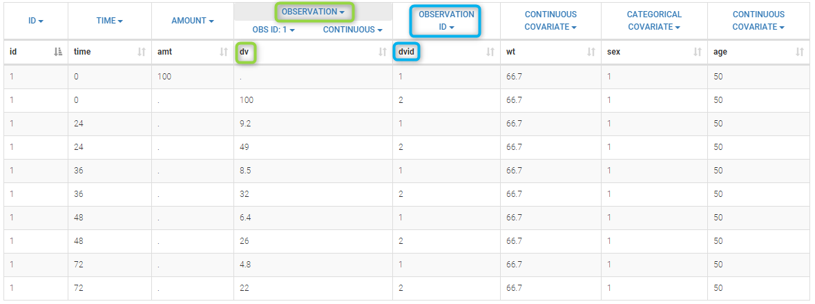
The column DV of the data file contains both the PK and the PD measurements: in Monolix this column is tagged as an OBSERVATION column. The column DVID is a flag defining the type of observation: DVID=1 for PK data and DVID=2 for PD data: the keyword OBSERVATION ID is then used for this column.
 We will use the model oral1_1cpt_TlagkaVCl from the
 Monolix PK library
[LONGITUDINAL]
input = {Tlag, ka, V, Cl}

EQUATION:
Cc = pkmodel(Tlag, ka, V, Cl)

OUTPUT:
output = {Cc}
Only the predicted concentration Cc is defined as an output of this model. Then, this prediction will be automatically associated to the outcome of type 1 (DVID=1) while the other observations (DVID=2) will be ignored.
Remark: any other ordered values could be used for OBSERVATION ID column: the smallest one will always be associated to the first prediction defined in the model.
Simultaneous PKPD modeling
- warfarin_PKPDimmediate_project (data = ‘warfarin_data.txt’, model = ‘immediateResponse_model.txt’)
It is also possible for the user to write his own PKPD model. The same PK model used previously and an immediate response model are defined in the model file immediateResponse_model.txt
[LONGITUDINAL]
input = {Tlag, ka, V, Cl, Imax, IC50, S0}

EQUATION:
Cc = pkmodel(Tlag, ka, V, Cl)
E = S0 * (1 - Imax*Cc/(Cc+IC50))

OUTPUT:
output = {Cc, E}
Two predictions are now defined in the model: Cc for the PK (DVID=1) and E for the PD (DVID=2).
- warfarin_PKPDeffect_project (data = ‘warfarin_data.txt’, model = ‘effectCompartment_model.txt’)
An effect compartment is defined in the model file effectCompartment_model.txt
[LONGITUDINAL]
input = {Tlag, ka, V, Cl, ke0, Imax, IC50, S0}

EQUATION:
{Cc, Ce} = pkmodel(Tlag, ka, V, Cl, ke0)
E = S0 * (1 - Imax*Ce/(Ce+IC50))

OUTPUT:
output = {Cc, E}
Ce is the concentration in the effect compartment
- warfarin_PKPDturnover_project (data = ‘warfarin_data.txt’, model = ‘turnover1_model.txt’)
An indirect response (turnover) model is defined in the model file turnover1_model.txt
[LONGITUDINAL]
input =  {Tlag, ka, V, Cl, Imax, IC50, Rin, kout}

EQUATION:
Cc = pkmodel(Tlag, ka, V, Cl)
E_0 = Rin/kout
ddt_E = Rin*(1-Imax*Cc/(Cc+IC50)) - kout*E

OUTPUT:
output = {Cc, E}
Sequential PKPD modelling
In the sequential approach, a PK model is developed and parameters are estimated in the first step. For a given PD model, different strategies are then possible for the second step, i.e., for estimating the population PD parameters:
Using estimated population PK parameters
- warfarin_PKPDseq1_project (data = ‘warfarin_data.txt’, model = ‘turnover1_model.txt’)
Population PK parameters are set to their estimated values but individual PK parameters are not assumed to be known and sampled from their conditional distributions at each SAEM iteration. In Monolix, this simply means changing the status of the population PK parameter values so that they are no longer used as initial estimates for SAEM but considered fixed as on the figure below.

To fix parameters, click on the green option button (framed in green) and choose the Fixed method as on the figure below

The joint PKPD model defined in turnover1_model.txt is again used with this project.
Using estimated individual PK parameters
- warfarin_PKPDseq2_project (data = ‘warfarinSeq_data.txt’, model = ‘turnoverSeq_model.txt’)
In htis case, individual PK parameters are set to their estimated values and used as constants in the PKPD model to fit the PD data. To do so, the individual PK parameters need to be added to the PD dataset (or PK/PD dataset) and tagged as regressors.
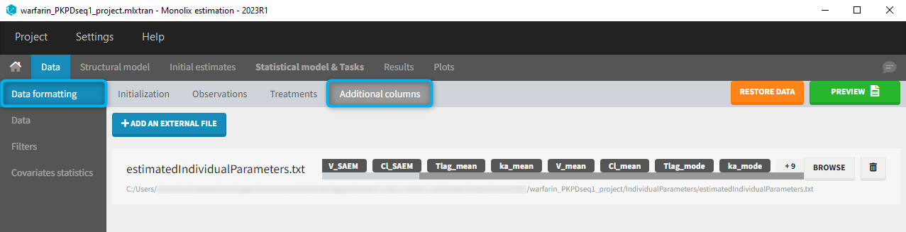
The PK project (that was executed before and through which the estimated PK parameters were obtained) contains in the result folder the individual parameter values “..\warfarin_PKPDseq1_project\IndividualParameters\estimatedIndividualParameters.txt”. These estimated PK parameters can be added to the PD dataset by using the data formatting tool integrated in Monolix version 2023R1. Depending which tasks have been run in the PK project, the individual parameters corresponding to the conditional mode (EBEs, with “_mode”), the conditional mean (mean of the samples from the conditional distributions, with “_mean”) and an approximation of the conditional mean obtained at the end of the SAEM step (with “_SAEM”) are available in the file. All columns are added to the PD dataset.
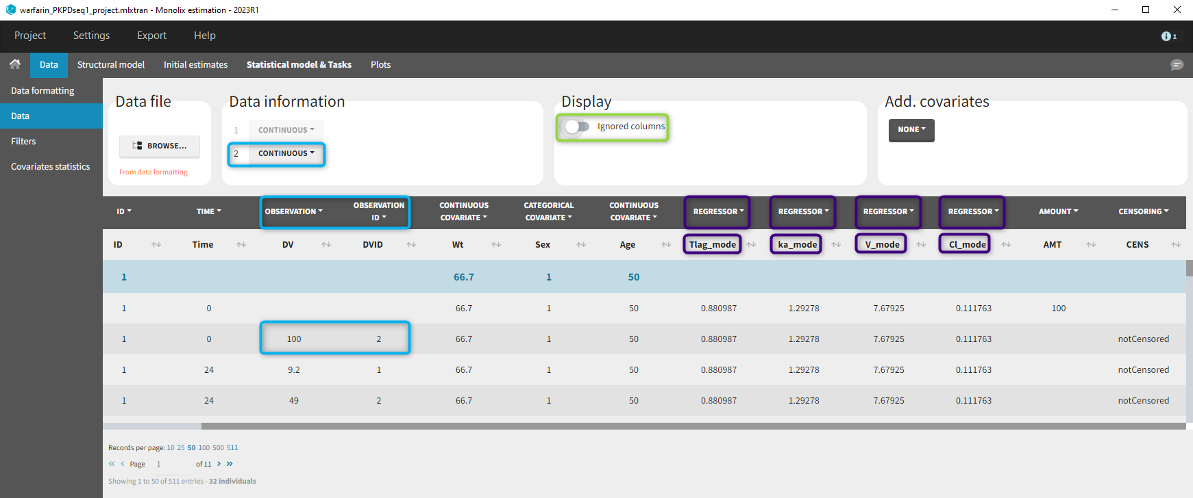
At the data tagging step, the user can choose which individual parameters to use. The most common is to use the EBEs so to tag the columns with “_mode” as regressor and leave the others as IGNORE (purple frame below). By activating the toggle button (green frame), the ignored columns flagged with the keyword IGNORE can be hidden.
We use the same turnover model for the PD data. Here, the PK parameters are defined as regression variables (i.e. regressors).
[LONGITUDINAL]
input =  {Imax, IC50, Rin, kout, Tlag, ka, V, Cl}
Tlag  = {use = regressor}
ka    = {use = regressor}
V     = {use = regressor}
Cl    = {use = regressor}

EQUATION:
Cc = pkmodel(Tlag,ka,V,Cl)
E_0 = Rin/kout
ddt_E= Rin*(1-Imax*Cc/(Cc+IC50)) - kout*E

OUTPUT:
output = {E}
As you can see, the names of the regressors do not match the parameter names. The regressors are matched by order (not by name) between the data set and the model input statement.
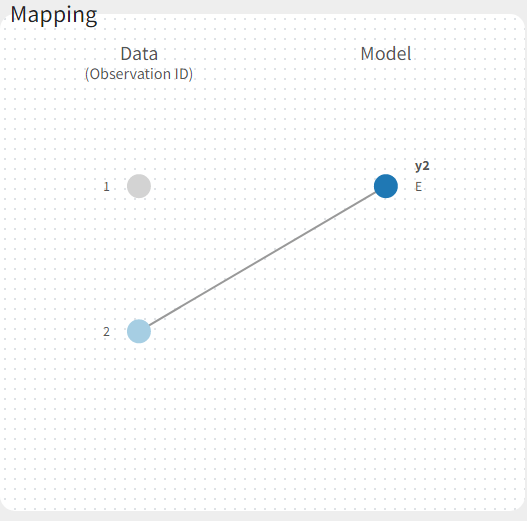
If there are multiple observation types in the data as well as different response vectors in the output statement of the structural model, then these must be mapped accordingly in the mapping panel.
Fitting a PKPD model to the PD data only
- warfarinPD_project (data = ‘warfarinPD_data.txt’, model = ‘turnoverPD_model.txt’)
In this example, only PD data is available. Nevertheless, a PKPD model – where only the effect is defined as a prediction – can be used for fitting this data and thus defined in the OUTPUT section.
[LONGITUDINAL]
input =  {Tlag, ka, V, Cl, Imax, IC50, Rin, kout}

EQUATION:
Cc = pkmodel(Tlag, ka, V, Cl)
E_0 = Rin/kout
ddt_E = Rin*(1-Imax*Cc/(Cc+IC50)) - kout*E

OUTPUT:
output = {E}
Case studies
- 8.case_studies/PKVK_project (data = ‘PKVK_data.txt’, model = ‘PKVK_model.txt’)
- 8.case_studies/hiv_project (data = ‘hiv_data.txt’, model = ‘hivLatent_model.txt’)