- Introduction
- Between subject mixture models
- Supervised learning (with regressor)
- Unsupervised learning (with bsmm function)
- Within subject mixture models
Objectives: learn how to implement between subject mixture models (BSMM) and within subject mixture models (WSMM).
Projects: bsmm1_project, bsmm2_project, wsmm_project
Introduction
There are two approaches to define a mixture of models:
- defining a mixture of structural models (via a regressor or via the bsmm function). This approach is detailed here.
- introducing a categorical covariate (known or latent). –> click here to go to the page dedicated to this approach.
Several types of mixture models exist, they are useful in the context of mixed effects models. It may be necessary in some situations to introduce diversity into the structural models themselves:
- Between-subject model mixtures (BSMM) assume that there exists subpopulations of individuals. Different structural models describe the response of each subpopulation, and each subject belongs to one of these subpopulations. One can imagine for example different structural models for responders, nonresponders and partial responders to a given treatment.
The easiest way to model a finite mixture model is to introduce a label sequence ")


")
$$f\left(t_{ij}; \psi_i, z_i \right) = \sum_{m=1}^M 1_{z_i = m} f_m\left( t_{ij}; \psi_i \right) $$
In other word, each subpopulation has its own structural model: 
- Within-subject model mixtures (WSMM) assume that there exist subpopulations (of cells, viruses, etc.) within each patient. In this case, different structural models can be used to describe the response of different subpopulations, but the proportion of each subpopulation depends on the patient.
Then, it makes sense to consider that the mixture of models happens within each individual. Such within-subject model mixtures require additional vectors of individual parameters ")
$$f\left( t_{ij}; \psi_i, z_i \right) = \sum_{m=1}^M \pi_{m,i} f_m\left( t_{ij}; \psi_i \right)$$
The proportions ")
Between subject mixture models
Supervised learning
- bsmm1_project (data = ‘pdmixt1_data.txt’, model = ‘bsmm1_model.txt’)
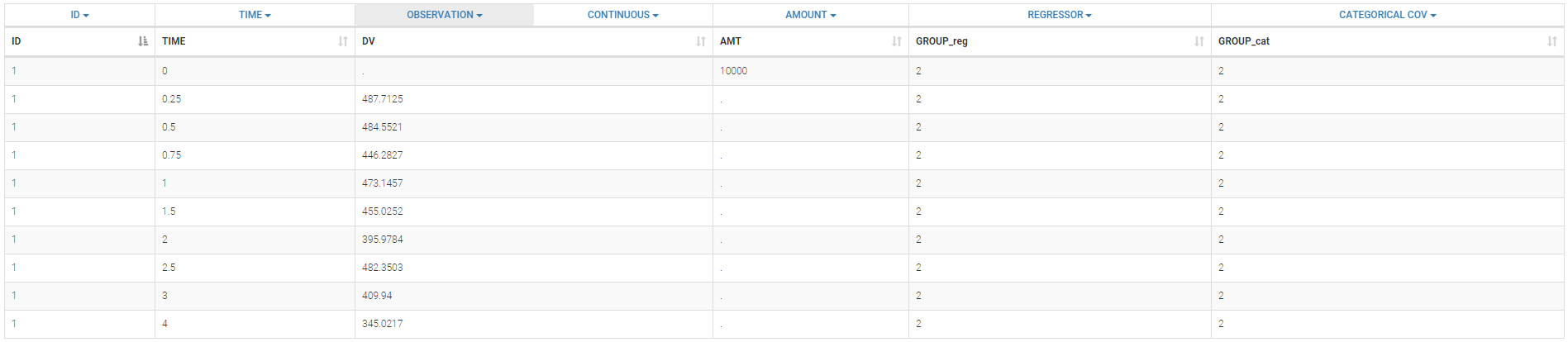
We consider a very simple example here with two subpopulations of individuals who receive a given treatment. The outcome of interest is the measured effect of the treatment (a viral load for instance). The two populations are non responders and responders. We assume here that the status of the patient is known. Then, the data file contains an additional column GROUP. This column is duplicated because Monolix uses it
- i) as a regression variable (REGRESSOR): it is used in the model to distinguish responders and non responders,
- ii) as a categorical covariate (CATEGORICAL COVARIATE): it is used to stratify the diagnosis plots.
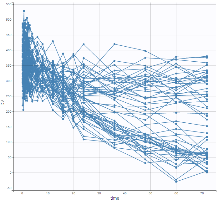
We can then display the data
and use the categorical covariate GROUP_CAT to split the plot into responders and non responders:
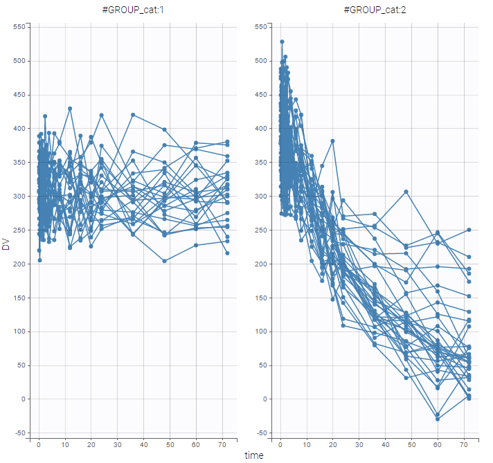 We use different structural models for non responders and responders. The predicted effect for non responders is constant f(t) = A1 while the predicted effect for responders decreases exponentially f(t) = A2 exp(-kt).
The model is implemented in the model file bsmm1_model.txt (note that the names of the regression variable in the data file and in the model script do not need to match):
[LONGITUDINAL]
input = {A1, A2, k, g}
g = {use=regressor}

EQUATION:
if g==1
   f = A1
else
   f = A2*exp(-k*max(t,0))
end

OUTPUT:
output = f
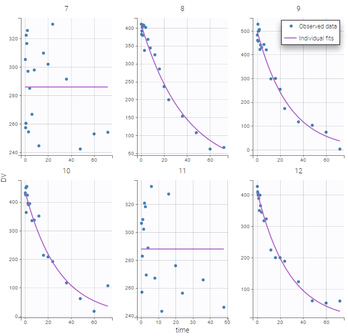
The plot of individual fits exhibit the two different structural models:
VPCs should then be splitted according to the GROUP_CAT
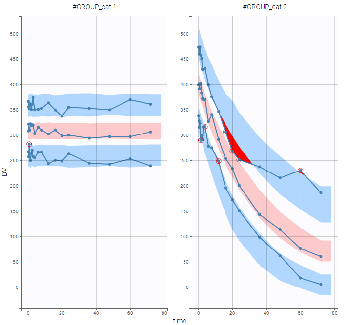
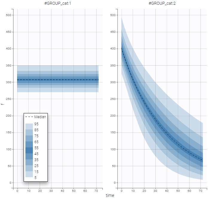
as well as the prediction distribution for non responders and responders:
Unsupervised learning
- bsmm2_project (data = ‘pdmixt2_data.txt’, model = ‘bsmm2_model.txt’)
The status of the patient is unknown in this project (which means that the column GROUP is not available anymore). Let p be the proportion of non responders in the population. Then, the structural model for a given subject is f1 with probability p and f2 with probability 1-p. The structural model is therefore a BSMM:
[LONGITUDINAL]
input = {A1, A2, k, p}

EQUATION:
f1 = A1
f2 = A2*exp(-k*max(t,0))
f  = bsmm(f1, p, f2, 1-p)

OUTPUT:
output = f
Important:
- The bsmm function must be used on the last line of the structural model, just before “OUTPUT:”. It is not possible to reuse the variable returned by the bsmm function (here f) in another equation.
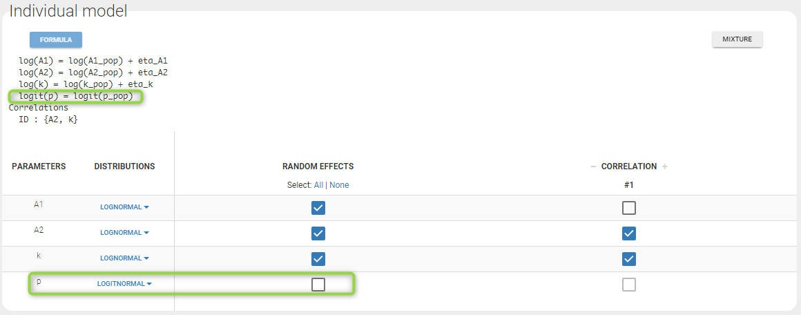
- p is a population parameter of the model to estimate. There is no inter-patient variability on p: all the subjects have the same probability of being a non responder in this example. We use a logit-normal distribution for p in order to constrain it to be between 0 and 1, but without variability:
 p is estimated with the other population parameters:
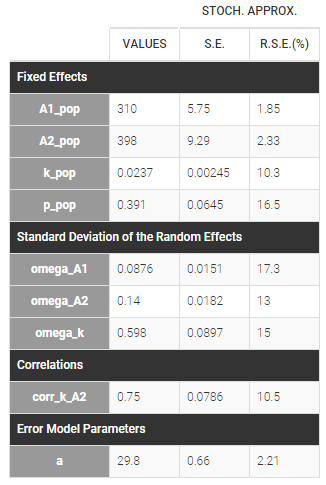
Then, the group to which a patient belongs is also estimated as the group of highest conditional probability:
$$\begin{aligned}\hat{z}_i &= 1~~~~\textrm{if}~~~~ \mathbb{P}(z_i=1 | (y_{ij}), \hat{\psi}_i, \hat{\theta})> \mathbb{P}(z_i=2 | (y_{ij}),\hat{\psi}_i, \hat{\theta}),\\ &=0~~~~\textrm{otherwise}\end{aligned}$$
The estimated groups can be used as a stratifying variable to split some plots such as VPCs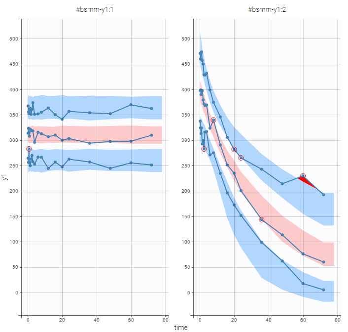
Bsmm function with ODEs
The bsmm function can also be used with models defined via ODE systems. The syntax in that case follows this example, with model M defined as a mixture of M1 and M2:
M1_0 = ... ; initial condition for M1
ddt_M1 = ... ; ODE for M1
M2_0 = ... ; initial condition for M2
ddt_M2 = ... ; ODE for M2

M = bsmm(M1,p1,M2,1-p1)
Unsupervised learning with latent covariates
If the models composing the mixture have a similar structure, it is sometimes possible and easier to implement the mixture with a latent categorical covariate instead of the bsmm function. It also has the advantage of allowing more than two mixture groups, while the bsmm function can only define two mixture groups.
Within subject mixture models
- wsmm_project (data = ‘pdmixt2_data.txt’, model = ‘wsmm_model.txt’)
It may be too simplistic to assume that each individual is represented by only one well-defined model from the mixture. We consider here that the mixture of models happens within each individual and use a WSMM: f = p*f1 + (1-p)*f2
[LONGITUDINAL]
input = {A1, A2, k, p}

EQUATION:
f1 = A1
f2 = A2*exp(-k*max(t,0))
f = wsmm(f1, p, f2, 1-p)

OUTPUT:
output = f
Remark: Here, writing f = wsmm(f1, p, f2, 1-p) is equivalent to writing f = p*f1 + (1-p)*f2
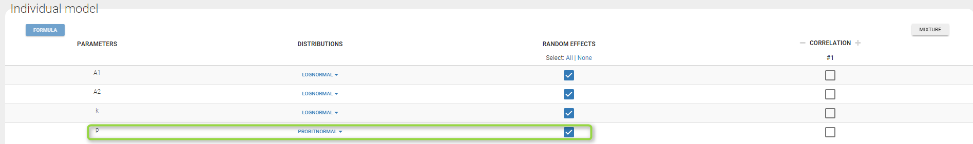
Important: Here, p is an individual parameter: the subjects have different proportions of non responder cells. We use a probit-normal distribution for p in order to constrain it to be between 0 and 1, with variability:
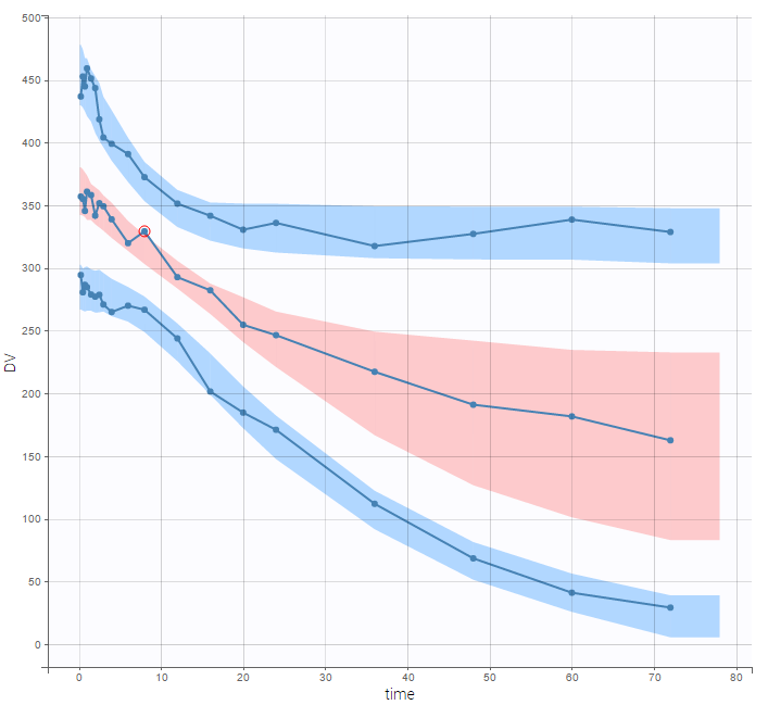
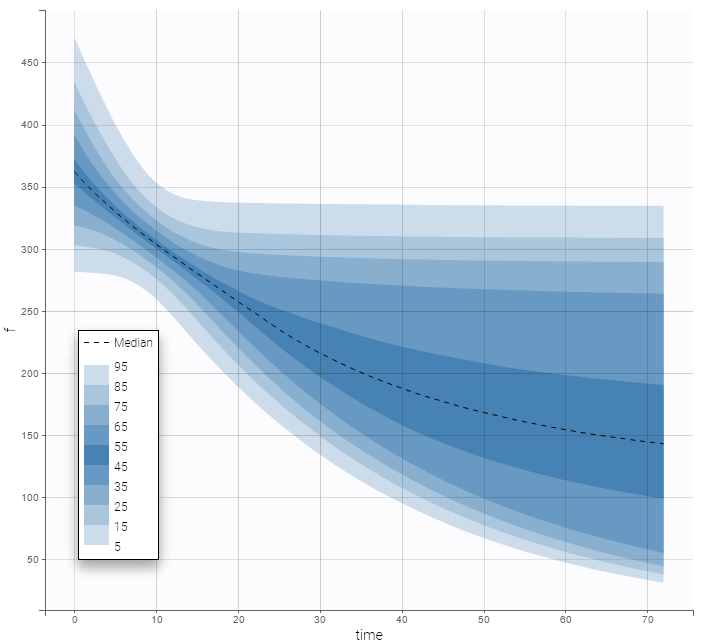
There is no latent covariate when using WSMM: mixtures are continuous mixtures. We therefore cannot split anymore the VPC and the prediction distribution anymore.
 |
 |
|---|