- Complex parameter-covariate relationships and time-dependent continuous covariates
- Categorical time-varying covariates
- Covariate-dependent parameter
- Covariate-dependent standard deviation
- Transforming a continuous covariate into a categorical covariate
Note that starting from version 2024 on, analytical solutions are used even if a time-varying regressor is used in the model.
Complex parameter-covariate relationships and time-dependent continuous covariates
Covariate-parameter relationships are usually defined via the Monolix GUI, leading for instance to exponential and power law relationships. However more complex parameter-covariate relationships such as Michaelis-Menten or Hill dependencies cannot the defined via the GUI because they cannot be put into the format where the (possibly transformed) covariate is added linearly on the transformed parameter. Similarly, when the covariate value is changing over time and thus not constant for each subject (or each occasion in each subject in case of occasions), the covariate cannot be added to the model via the GUI. In both cases, the effect of the covariate must be tagged as a regressor and the relationship must be defined directly in the model file.
In the following, we will use as an example a Hill relationship between the clearance parameter Cl and the time-varying post-conception age (PCA) covariate, which is a typical way to scale clearance in paediatric pharmacokinetics:
$$Cl_i = Cl_{pop} \frac{PCA^n}{PCA^n+A50^n} e^{\eta_i}$$
where \(Cl_i\) is the parameter value for individual i, \(Cl_{pop}\) the typical clearance for an adult, \(A50\) the PCA for the clearance to reach 50% mature, \(n\) the shape parameter and \(\eta_i\) the random effect for individual i.
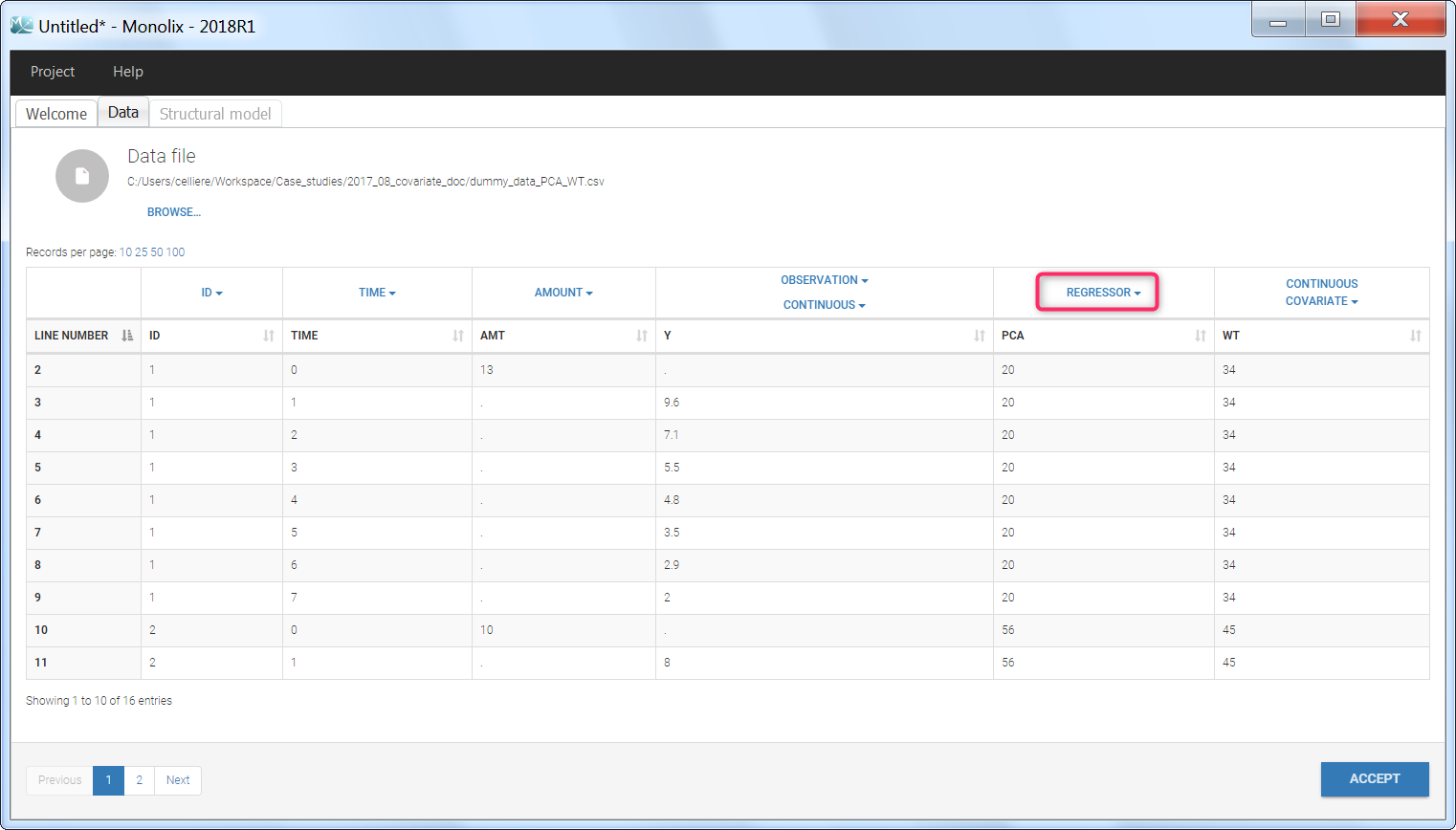
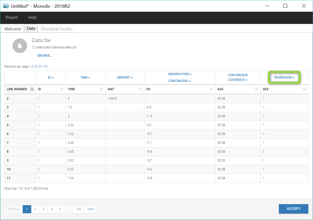
Step 1: To make the PCA covariate available as a variable is the model file, the first step is to tag it as a regressor column-type REGRESSOR when loading the data set (instead of using the CONTINUOUS COVARIATE column-type).
Step 2: In the model file, the PCA covariate is passed as input argument and designated as being a regressor. The clearance Cl, the hill shape parameter n, and the A50 are passed as usual input parameters:
[LONGITUDINAL]
input = {..., Cl, n, A50, PCA, ...}
PCA = {use=regressor}
If several regressors are used, be careful that the regressors are matched by order with the data set columns tagged as REGRESSOR (not by name).
The relationship between the clearance Cl and the post-conception age PCA is defined in the EQUATION: block, before ClwithPCA is used (for instance in a simple (V,Cl) model):
EQUATION:
ClwithPCA = Cl * PCA^n / (PCA^n + A50^n)

Cc = pkmodel(Cl=ClwithPCA, V)
Note that the input parameter Cl includes the random effect ( \(Cl = Cl_{pop} e^{\eta_i} \) ), such that only the covariate term must be added. Because the parameter including the covariate effect CLwithPCA is not a standard keyword for macros, one must write Cl=ClwithPCA.
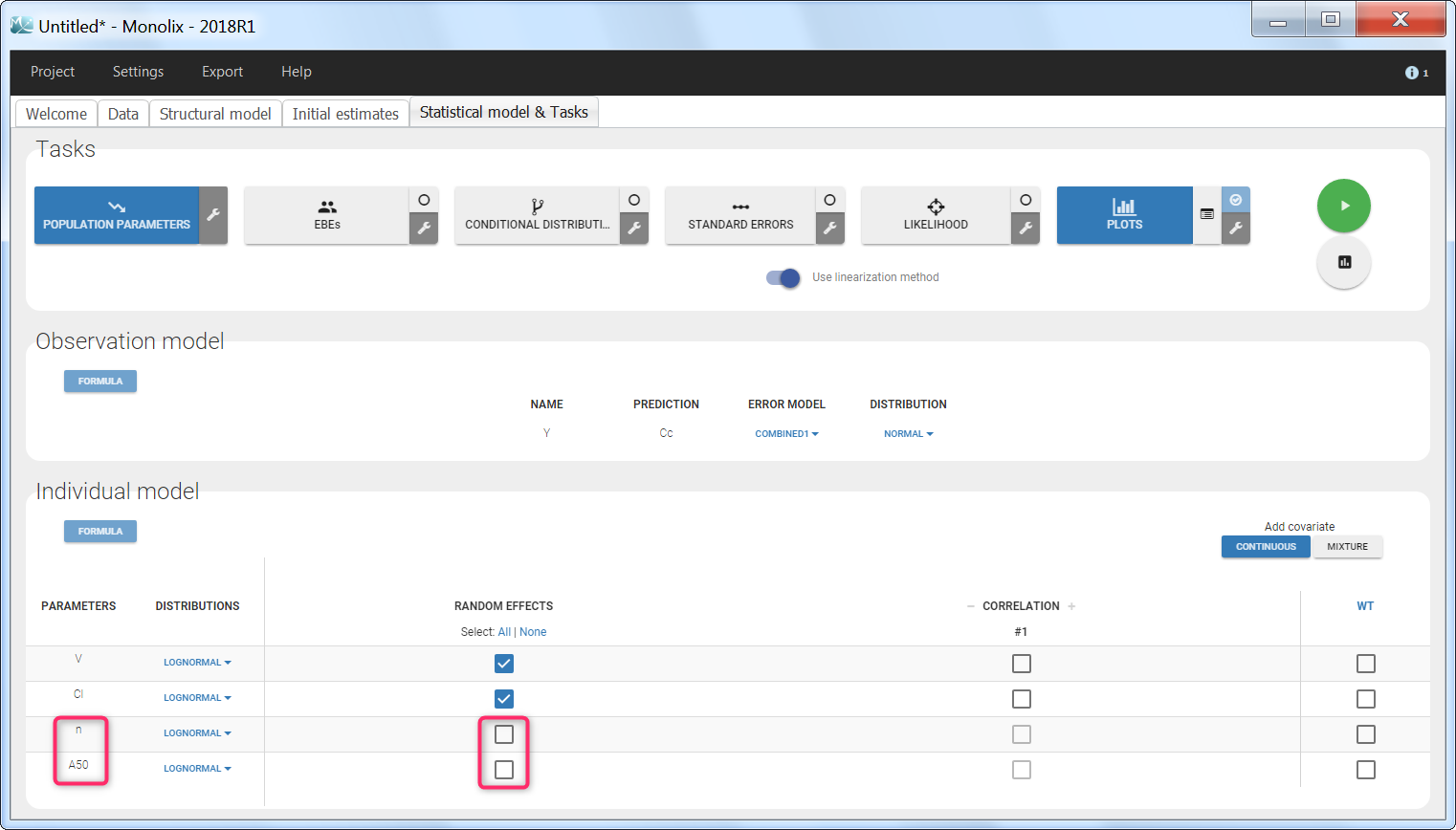
Step 3: The definition of the parameters in the GUI deserves special attention. Indeed the parameters n and A50 characterize the covariate effect and are the same for all individuals: their inter-individual variability must be removed by unselecting the random effects. On the opposite, the parameter Cl keeps its inter-individual variability, corresponding to the \(e^{\eta_i} \) term.
Step 4: When covariates relationships are not defined via the GUI, the p-value corresponding to the Wald test is not automatically outputted. It is however possible to calculate it externally. Assuming that we would like to test if the shape parameter n is significantly different from 1:
$$H_0: \quad \textrm{”}n=1\textrm{”} \quad \textrm{versus} \quad H_1:\quad \textrm{”}n \neq 1\textrm{”}$$
Using the parameter estimate and the s.e outputted by Monolix, we can calculate the Wald statistic:
$$W = \frac{\hat{n}-n_{ref}}{\textrm{s.e}(\hat{n})}$$
with \(\hat{n}\) the estimated value for parameter n, \(n_{ref}\) the reference value for n (here 1) and \(\textrm{s.e}(\hat{n}) \) the standard error for the n estimate.
The test statistic W can then be compared to a standard normal distribution. Below we propose a simple R script to calculate the p-value:
 n_estimated = 1.32
 n_ref = 1
 se_n = 0.12

 W = abs(n_estimated - n_ref)/se_n

 pvalue = 2 * pnorm(W, mean = 0, sd = 1, lower.tail = FALSE)
Note that the factor 2 is added to do a two-sided test.
Categorical time-varying covariates
Categorical covariates may also be time-varying, for instance when the covariate represents concomitant medications over the course of the clinical trial or a fed/fasting state at the time of the dose.
In the following, we will use as an example a concomitant medication categorical covariate with 3 categories: no concomitant drug, concomitant drug 1, and concomitant drug 2. We would like to investigate the effect of the concomitant drug covariate on the clearance Cl.
$$Cl_i = \begin{cases}Cl_{pop} e^{\eta_i} & \textrm{if no concomitant drug} \\ Cl_{pop} (1+\beta_1)e^{\eta_i} & \textrm{if concomitant drug 1} \\ Cl_{pop} (1+\beta_2)e^{\eta_i} & \textrm{if concomitant drug 2} \end{cases}$$
where \(Cl_i\) is the parameter value for individual i, \(Cl_{pop}\) the typical clearance if no concomitant drug, \(\beta_1\) the fractional change in case of concomitant drug 1, \(\beta_2\) the fractional change in case of concomitant drug 2 and \(\eta_i\) the random effect for individual i.
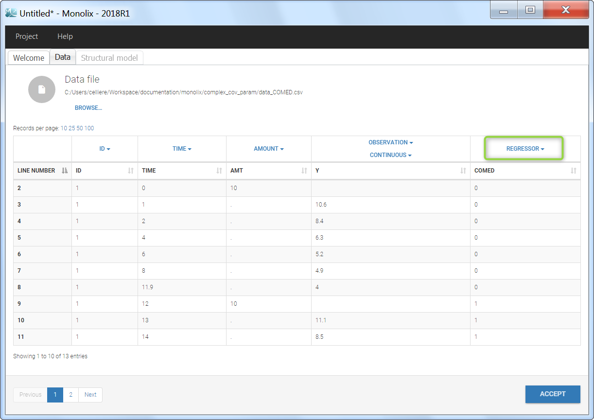
Step 1: Encode the categorical covariate as integers. Indeed, while strings are accepted for the CATEGORICAL COVARIATE column-type, only numbers are accepted for the REGRESSOR column-type. Here we will use 0 = no concomitant medication, 1 = concomitant drug 1 and 2 = concomitant drug 2.
Step 2: To make the COMED covariate available as a variable is the model file, tag it as a column-type REGRESSOR when loading the data set (instead of using the CATEGORICAL COVARIATE column-type).
Step 3: In the model file, the COMED covariate is passed as input argument and designated as being a regressor. The clearance Cl, and the two beta parameters are passed as usual input parameters:
[LONGITUDINAL]
input = {..., Cl, beta1, beta2, COMED, ...}
COMED = {use=regressor}
If several regressors are used, be careful that the regressors are matched by order with the data set columns tagged as REGRESSOR (not by name).
To define the COMED covariate impact, we use a if/else statement in the EQUATION: block. The parameter value taking into account the COMED effect (called ClwithCOMED in this example) can then be used in an ODE system or within macros.
EQUATION:
if COMED==0
ClwithCOMED = Cl
elseif COMED==1
ClwithCOMED = Cl * (1+beta1)
else
ClwithCOMED = Cl * (1+beta2)
end

Cc = pkmodel(Cl=ClwithCOMED, V)
Note that the input parameter Cl includes the random effect ( \(Cl = Cl_{pop} e^{\eta_i} \) ), such that only the covariate term must be added. Because the parameter including the covariate effect CLwithCOMED is not a standard keyword for macros, one must write Cl=ClwithCOMED.
If the categorical covariate has only two categories encoded as 0 and 1 (for instance COMED=0 for no concomitant medication and COMED=1 for concomitant medication), it is also possible to write the model in a more compact form:
ClwithCOMED = Cl * (1 + beta * COMED)
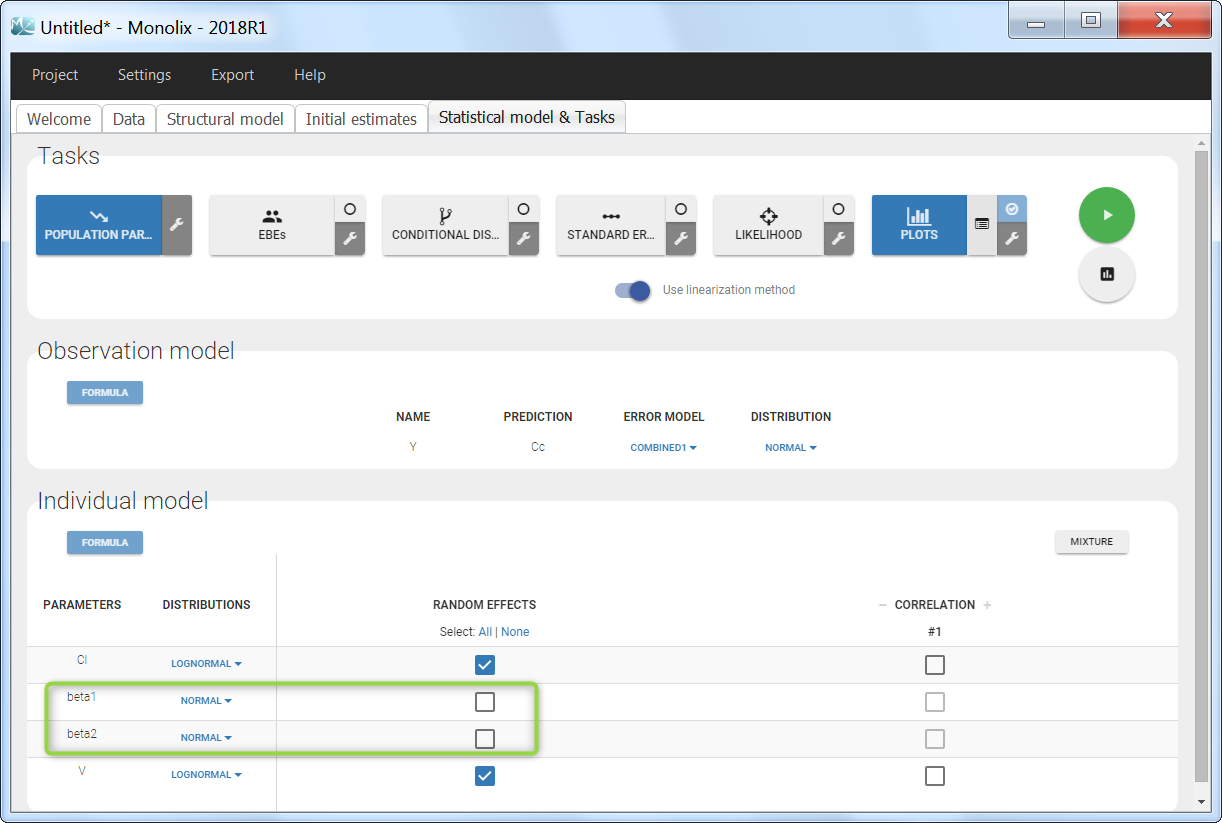
Step 4: The definition of the parameters in the GUI deserves special attention. Indeed the parameters beta1 and beta2 characterize the covariate effect and are the same for all individuals: their inter-individual variability must be removed by unselecting the random effects. On the opposite, the parameter Cl keeps its inter-individual variability, corresponding to the \(e^{\eta_i} \) term. In addition, we choose a normal distribution for beta1 and beta2 (with a standard deviation of zero as we have removed the random effects) in order to allow both positive and negative values.
Covariate-dependent parameter
When adding a categorical covariate on a parameter via the GUI, different typical values will be estimated for each group. However, all groups will have the same standard deviation. It can sometimes be useful to consider that the standard deviations also differ between groups. For example, healthy volunteers may have a smaller inter-individual variability than patients.
From the 2018R1 version on, categorical covariates affecting both the typical value and the standard deviation have to be defined directly in the structural model, by using the covariate as a regressor and different parameters depending on the value of the regressor. Using a different parameter for each group permits to estimate a typical value and a standard deviation per group. Note that a regressor can contain only numbers, so the categorical covariate should be encoded with integers rather than strings.
We show below an example, where the fixed effect and standard deviation of the volume V both depend on the covariate SEX. This require the definition of two different parameters VM (for male) and VF (for female).
Step 1: To make the covariate SEX available as a variable is the model file, it has to be tagged as a regressor with column-type REGRESSOR when loading the data set (instead of using the CONTINUOUS COVARIATE and CATEGORICAL COVARIATE column-types).
Step 2: In the model file shown below, the covariate SEX is passed as input argument and designated as being a regressor. Two parameters VM (for male) and VF (for female) are given as input, to be used as the volume V depending on the SEX. The use of VM or VF depending on the SEX value is defined in the EQUATION: block, before V is used (for instance in a simple (V,Cl) model):
[LONGITUDINAL]
input = {Cl, VM, VF, SEX}
SEX = {use=regressor}
EQUATION:
if SEX==0
V = VM
else
V = VF
end

Cc = pkmodel(Cl, V)

OUTPUT:
output = {Cc}
Step 3: The distribution of the parameters VM and VF is set as usual in the GUI. A different typical population value and a different standard deviation of the random effects will be estimated for males and females.
Note: As SEX has been tagged as a regressor, it is not available as a covariate in the GUI. If a covariate effect of SEX on another parameter is needed, the column SEX can be duplicated in the dataset so that the duplicate can be tagged as a covariate.
Covariate-dependent standard deviation
This video shows a variation of the previous solution, where only the standard deviation of the random effect of a parameter is covariate-dependent, while the fixed effect is not affected.
Transforming a continuous covariate into a categorical covariate
The Monolix GUI allows to discretize a continuous covariate in order to handle it as a categorical covariate in the model, using binary 0/1 values.