The construction of a VPC plot for time-to-event data in Monolix requires several steps:
- 1. Simulation of datasets. First, Monolix simulates datasets using the population model, which contains the structural and statistical models and the estimated population parameters.
- 2. Survival function estimators. Then, for the original dataset and each simulated dataset, it estimates the survival function with either the Kaplan-Meier estimator for exactly observed events or the Turnbull estimator for interval censored events.
- 3. Prediction interval. Finally, Monolix calculates lower and upper percentiles of the simulated survival function estimates, which give a prediction interval.
1. Simulation of TTE data sets using a population model
Simulations of time-to-event datasets give, for each individual, times when an event occurs. The simulations are based on the same design as in the original data set, the same number of individuals as in the original data set and individual parameters are sampled using the covariates from this original data set and the population parameters estimated in Monolix.
To simulate a time when an event occurs, (u) is defined as a probability that an event (X) occurs before a certain time (T). This probability is computed using the cumulative hazard function (H(t))
 = 1-exp\left(-\int_0^T h(t,\psi_i) dt\right) = 1-exp(-H(T)),")
where \(H\) is a solution to the ODE system \(dH/dt = h\). A value of the probability \(u\) is sampled from the uniform \([0,1]\) distribution, thus in the above equation the time T becomes the unknown variable. A root finding method from an ODE solver finds its value.
The time T is not a given independent variable, but it is a simulated observation. Moreover, simulations are only until the time \(T_{max}\), which corresponds to the last time found in the data set. This value is the final integration time of the ODEs for each individual and it also defines a unique right censoring time for all individuals in the simulated data sets. It is independent of the individual times of events or right censoring in the original data set.
If the simulation fails because of a numerical error (e. g. because of a too high hazard), the simulated individuals with NaNs in their simulations are not used in the prediction interval, and the proportion of simulated individuals involved is then displayed in the interface.
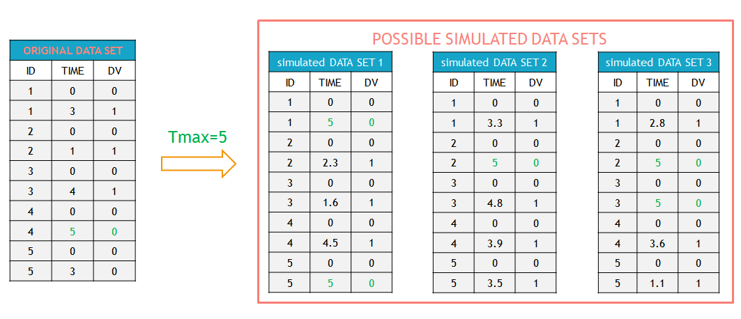
Example
In this example, the individual 3 in the original data set (table on the left) experienced an event at time 4. In the simulations (tables on the right), an event for this individual can occur before or after that time, or may occur after \(T_{max}=5\) (last table). Similarly, while the individual 5 left the study at time 3 without experiencing an event in the original data set, in the simulations for this individual an event can occur before or after time 3. If an event has not occurred at \(T_{max}=5\), then it is right censored.
Possible sources of bias in the simulations
Censoring (dropout)
In the original dataset (input Monolix dataset), censoring can be at any time: because the patient drops out or because the study is stopped for instance. In contrast, simulated datasets have no dropout until the global Tmax over all individuals, which means that there are on average more events in the simulated datasets than in the original dataset. However, if censoring in the original dataset is truly random, simulating until the global Tmax over all individuals should not produce a bias because the “additional” simulated events are evenly distributed over time. But if censoring in the dataset is not truly random, the empirical Kaplan-Meier curve is biased while the VPC predictions are not, so it may appear as a misfit. If we would instead censor the simulated datasets at the same censoring times as in the original dataset (Tmax=5 for id 4 and Tmax=3 for ID 5 on the above example), this could introduce other bias.
Regressor
If the TTE model depends on a regressor, the regressor is interpolated using last value carried forward.
Doses
If the TTE model depends on a PK model with doses present in the dataset, it is important to also include the planned (but not given because of event or dropout) doses in the dataset such that the doses span the same time range for all individuals. Otherwise this will create a bias in the VPC.
2. Survival function estimators
Given some survival data that includes censoring (right-censoring or interval-censoring), a survival function can be estimated as a non-parametric maximum likelihood estimator (NPMLE).
Thus Monolix estimates an NPMLE for each simulated dataset, depending on the event type:
- Kaplan-Meier estimator for exactly observed events.
- Turnbull estimator for interval censored data.
The calculation of these estimators is detailed in the next sections.
Note: for interval censored data, the Turnbull estimator is used only in the VPC:
- In the plot of Observed data, Monolix assumes that all events are exactly observed and displays the data using the Kaplan-Meier estimator explained in the previous section. This is because that plot is generated right after accepting the dataset, before a model has been selected. However, just looking at the dataset, the case of exact and interval censored events are indistinguishable. For example: assume that an observation period started at \(t=0\) and at \(t=1\) an event is marked by 1 in the column for the observation. Without any other information, the event could have occurred at \(t=1\) or before.
- In the VPC, Monolix uses the eventType information specified in the structural model. If “eventType = intervalCensored” is specified in the structural model, Monolix uses the Turnbull estimator for empirical and simulated survival curves in the VPC, in order to avoid bias in the survival function estimate. If eventType is not specified in the structural model, Monolix considers all interval-censored events as exactly observed at the end of a censored interval, and uses the Kaplan-Meier estimator.
DEFINITION:
Event = {type = event, eventType = intervalCensored, intervalLength = L,
                maxEventNumber = 1, hazard = h}
2.1. Exact events: Kaplan-Meier estimator
The Kaplan-Meier estimator, or product limit estimator, is a type of non-parametric maximum likelihood estimator and a standard method to approximate the survival function \( S(t) \) in the case of exact events. It describes the probability that an individual survives until time t, knowing that it survived at any earlier time. For single events, it is given by the following formula:
=\prod_{i:t_i<t} \left(1-\frac{d_i}{n_i}\right),")
where
- \(t_i\) – times before t, when at least one event occurred,
- \(d_i\) – number of events at the time \(t_i\),
- \(n_i\) – number of individuals at risk, that is who did not experience an event until \(t_i\).
The probability \((p_e)\) of an event is the ratio between the number of occurred events \((d_i)\) and the number of individuals at risk \((n_i)\). The complement of it, \((1-p_e)\), gives an estimation of the survival. For each time t, the total number of individuals at risk, who survived, may change. Thus, the current survival probability is the product of all probabilities at previous times \(t_i\), when at least one event occurred.
This formula can be better understood by calculating for example the probability that a patient survives 2 days: it is a product of two probabilities: the probability that the patient survives the first day and a conditional probability that they survive the second day, knowing that they survived the first one.
Example:
On the left of the figure below, a typical example of a time-to-event data set contains information about exact times when individuals experienced an event (T=1) or when they left the study (drop-out: T=0). Five individuals have two observations each: the time at which the observation starts (T=0 for everyone) and the time of an event. If a patient leaves the study, then the dataset contains a drop-out time with T=0, instead of T=1, in the column for the observations. This means that the patient experienced no event but survived until the drop-out time. The Kaplan-Meier estimator takes into account such situations, because these individuals are not counted as individuals at risk (they are not counted in the denominator \(n_i\)) at later times.
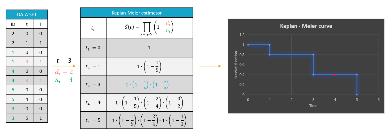
The study starts at time \(t_1\). There are no events, so \(d_1=0\) and the value of the Kaplan-Meier estimator is 1. Until the next event time at \(t_2=1\), the estimator remains constant. At that time, one individual experienced an event, hence \(d_2=1\), and all individuals survived until that time so \(n_2=5\). As a result, the probability to survive decreases by 0.2. It is the height of the jump at \(t=1\) in the plot. The Kaplan-Meier estimator remains constant until the next event. At time \(t=3\) there are two events. The number \(n_3\) counts now only 4 individuals – it has decreased by 1 due to the previous event. The final probability at time 3 is a product of all earlier probabilities. At \(t=4\) there is a drop-out: patient 5 left the study without experiencing an event. The survival curve remains constant and a red dot marks the drop-out. The Kaplan-Meier estimator takes into account this situations, because at the next event time \(t=5\), this individual is not counted as an individual at risk – thus the denominator n will be smaller. Finally, at time \(t=5\), there is only one individual left, and one event, so the survival becomes 0.
Remarks
- The Kaplan-Meier estimator handles correctly the information about individuals who left the study (right-censoring), but there is a bias when the exact times of events are unknown (interval-censoring).
- In the TTE VPC, Monolix estimates a linear approximation of the Kaplan-Meier estimate.
2.2 Interval censored events: Turnbull estimator
The Turnbull estimator is a generalization of the Kaplan-Meier estimator that allows for interval censoring. In the TTE VPC, Monolix uses this estimator to plot both the empirical and simulated survival curves.
Interval censored events do not occur at exact times \( t_i \), \(i = (1,…,n) \), but within some time intervals between times \( L_i \) and \( U_i \), \( L_i < t_i \leq U_i \). In case of right censored data (dropout), \( L_i\) is the time when the individual leaves the study, and \( U_i = +\infty \): an event will occur within the interval \( (L_i, +\infty) \).
In the TTE VPC, the intervals \( (L_i, U_i] \) are:
-
- For the empirical survival curve, they correspond to the censoring intervals of the original data set.
- For simulated survival curves, the definition of these intervals depends on whether the structural model contains the option “intervalLength” or not:
- If “intervalLength=L” is given, then the intervals are \([0, L], (L, 2\cdot L],\dots , (m\cdot L,T_{max} ]\)
- If “intervalLength” is missing, then the whole period of observation defined with the minimal and maximal times in the data is split in 10 regular intervals.
Note: Simulations of interval censored datasets give, as in the case of exactly observed events, exact times of events for each individual. In order to compare the simulated survival to the empirical survival without bias, simulated events are counted in regular intervals to be transformed into interval censored events, and they are then represented in the VPC with the Turnbull estimator just like for the empirical survival.
Turnbull intervals
The Turnbull estimator is computed on time intervals \( (\tau_{j-1} , \tau_j] \) that are called Turnbull intervals:

This grid of times is constructed from all points \( L_i, U_i \) for \( i = 1,…,n\) in increasing order.
Turnbull algorithm
Notations
- The probability that an event occurs in a j-th Turnbull interval is
- For each individual \( i\): \( \alpha_i \) denotes a weight such that
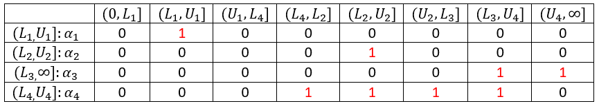
The Weight \(\alpha_{ij} \) is an event indicator – it indicates whether an event from the interval \( (L_i, U_i] \) occurred at \( \tau_j \).
- \(d_j\) is the number of events until \(\tau_j\) and \(n_j\) is the number of individuals at risk at \(\tau_j\)
- The likelihood function for \(p = (p_1, …, p_{m+1})\) is:
 = S(\tau_{j-1}) - S(\tau_j)")
![\alpha_i = 1\cdot { (\tau_{j-1} , \tau_j] \subset (L_i, U_i] }.](http://s0.wp.com/latex.php?latex=+%5Calpha_i+%3D+1%5Ccdot+%7B+%28%5Ctau_%7Bj-1%7D+%2C+%5Ctau_j%5D+%5Csubset+%28L_i%2C+U_i%5D+%7D.&bg=ffffff&fg=000&s=0 "\alpha_i = 1\cdot { (\tau_{j-1} , \tau_j] \subset (L_i, U_i] }.") The Weight \(\alpha_{ij} \) is an event indicator – it indicates whether an event from the interval \( (L_i, U_i] \) occurred at \( \tau_j \).
The Weight \(\alpha_{ij} \) is an event indicator – it indicates whether an event from the interval \( (L_i, U_i] \) occurred at \( \tau_j \).![L_S(p)= \prod_{i-1}^n [S(L_i) - S(R_i)] = \prod_{i-1}^n\sum_{j=1}^{m+1}\alpha_{ij} p_j](http://s0.wp.com/latex.php?latex=L_S%28p%29%3D+%5Cprod_%7Bi-1%7D%5En+%5BS%28L_i%29+-+S%28R_i%29%5D+%3D+%5Cprod_%7Bi-1%7D%5En%5Csum_%7Bj%3D1%7D%5E%7Bm%2B1%7D%5Calpha_%7Bij%7D+p_j&bg=ffffff&fg=000&s=0 "L_S(p)= \prod_{i-1}^n [S(L_i) - S(R_i)] = \prod_{i-1}^n\sum_{j=1}^{m+1}\alpha_{ij} p_j")
Main idea of the Turnbull algorithm
Finding the NPMLE of S, denoted by \(\hat{S}\), means maximizing \(L_S(p)\) under the constraint that \(p_j\) are positive and \(\sum_{j=1}^{m+1} p_j = 1\). The original Turnbull algorithm (1976) is the first and the simplest method to maximize \(L_S(p)\) with respect to \(p\). It is an application of the Expectation-Maximisation (EM) algorithm.
Remark: \(L_S\) depends only on values of S at points \(\tau_j\), and the behaviour of S within the Turnbull intervals is unknown. The convention applied here is: \(\hat{S}(t) = \hat{S}(\tau_j)\) when \(\tau_{j-1}\leq t\leq \tau_j\).
Procedure
The algorithm is the following:
- Step 0: Initialization – choose an initial guess for \( S^{old}(\tau_j) \). This initial guess for S is the estimate obtained from the Kaplan-Meier estimator under the assumption that events occur at \( U_i \), interpolated on the \( \tau – \) grid.
- Step 1: Compute the probability of an event at time \( \tau_j \) as
 - S^{old}(\tau_j), j = 1,\dots ,m")
- Step 2: Estimate the number of events at \( \tau_j \) as

- Step 3: Compute the estimated number of individuals at risk at time \( \tau_j \)

- Step 4: Compute \(S^{new} \) using the Kaplan-Meier estimator using \( \tilde(d) \) and \( \tilde(n) \) to update the survival function
- Stopping criterion: If the updated solution \(S^{new} \) is close to the old solution \(S^{old} \) (in Monolix, \(\Vert S^{new} – S^{old} \Vert < 0.001\) ), stop, otherwise set \(S^{old} = S^{new} \) and repeat steps 1 – 4
Linear approximation
In the TTE VPC, just like for the the Kaplan-Meier estimate, Monolix calculates a linear approximation of the Turnbull estimate.
Example
Below we show a small dataset with interval censored events. The individuals are in increasing order of the times at which censored intervals end. The figure on the rights shows two curves:
- The upper bound curve is the Kaplan-Meier estimate assuming that events occur exactly at the upper interval limit \( t_i = U_i \).
- The lower bound curve is the Kaplan-Meier estimate assuming that events occur exactly at the lower interval limit \( t_i = L_i \).

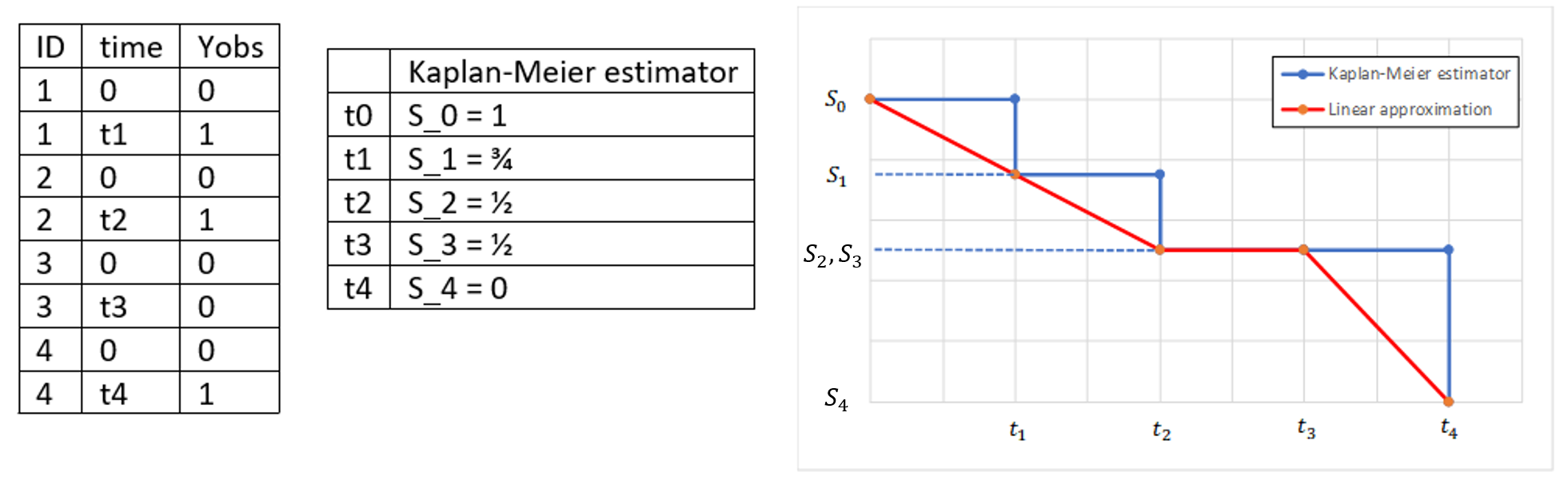
For comparison, we show now a similar dataset corresponding to exactly observed events at the upper interval limit. The figure on the right shows again the Kaplan-Meier estimator, and in addition its linear approximation.
Procedure
The time points of the lower and upper interval limits for all individuals are ordered in increasing sequence. In this example, the assumption is


The Turnbull intervals are the intervals \( (\tau_{j-1},\tau_j]\), where \(j=1,\dots , m\), with \(\tau_0=0\) and \(\tau_8=\infty\).
The weights \( \alpha_{ij} \) are elements of the following matrix:
First iteration of the algorithm
Step 0: The initial guess is the upper bound curve, that is the Kaplan-Meier estimator under the assumption that events occur at \( U_i \), interpolated on the \( \tau – \) grid.
=1,\quad S^{old}(\tau_1)=1,\quad S^{old}(\tau_2)=S_1,\quad S^{old}(\tau_3)=S_1,\quad S^{old}(\tau_4)=S_1\newline S^{old}(\tau_5)=S_2,\quad S^{old}(\tau_6)=S_2,\quad S^{old}(\tau_7)=S_4,\quad S^{old}(\tau_8)=S_4")
Step 1: The probabilities that events occur in the Turnbull intervals are

Step 2: Modified number of events
\(\quad\quad\quad \tilde{d}_1=0\\
\quad\quad\quad\tilde{d}_2=\frac{\alpha_{12} p_2}{\alpha_{12} p_2 }=1\\
\quad\quad\quad\tilde{d}_3=0\\
\quad\quad\quad\tilde{d}_4=0\\
\quad\quad\quad\tilde{d}_5=\frac{\alpha_{25} p_5}{\alpha_{25} p_5 } + \frac{\alpha_{45} p_5}{\alpha_{45} p_5+\alpha_{47} p_7 }=1+\frac{S_1-S_2}{S_1-S_4 }\\
\quad\quad\quad\tilde{d}_6=0\\
\quad\quad\quad\tilde{d}_7=\frac{\alpha_{37} p_7}{\alpha_{37} p_7 } + \frac{\alpha_{47} p_7}{\alpha_{45} p_5+\alpha_{47} p_7 } =1+\frac{S_2-S_4}{S_1-S_4 }\\
\quad\quad\quad\tilde{d}_8=0\)
Step 3: Modified number of individuals at risk
\(\quad\quad\quad\tilde{n}_1=4\\
\quad\quad\quad\tilde{n}_2=4\\
\quad\quad\quad\tilde{n}_3=3\\
\quad\quad\quad\tilde{n}_4=3\\
\quad\quad\quad\tilde{n}_5=3 \\
\quad\quad\quad\tilde{n}_6=1+\frac{S_2-S_4}{S_1-S_4}\\
\quad\quad\quad\tilde{n}_7=1+\frac{S_2-S_4}{S_1-S_4}\\
\quad\quad\quad\tilde{n}_8=0\)
Step 4: Kaplan-Meier estimator for the modified values of \(d\) and \(n\):
\(\quad\quad\quad S^{new}(\tau_0)=1\\
\quad\quad\quad S^{new}(\tau_1) = 1\cdot (1-\frac{0}{4})=1\\
\quad\quad\quad S^{new}(\tau_2) = 1\cdot (1-\frac{1}{4})=\frac{3}{4}\\
\quad\quad\quad S^{new}(\tau_3) = \frac{3}{4}\cdot (1-\frac{0}{3}) = \frac{3}{4}\\
\quad\quad\quad S^{new}(\tau_4) = \frac{3}{4}\cdot (1-\frac{0}{3}) = \frac{3}{4}\\
\quad\quad\quad S^{new}(\tau_5) = \frac{3}{4}\cdot (1-\frac{1+\frac{1}{3}}{3}) = \frac{5}{12}\\
\quad\quad\quad S^{new}(\tau_6) = \frac{5}{12}\cdot (1-\frac{0}{1+\frac{2}{3}}) = \frac{5}{12}\\
\quad\quad\quad S^{new}(\tau_7) = \frac{5}{12}\cdot (1-\frac{1+\frac{2}{3}}{1+\frac{2}{3}}) = 0\\
\quad\quad\quad S^{new}(\tau_8) = 0\)
The figure below compares the linear approximations of Turnbull estimate at the start of the first iteration (\(S^{old}\)) and at the end (\(S^{new}\)), as well as the linear approximation of the Kaplan-Meier estimate in case of exact events.
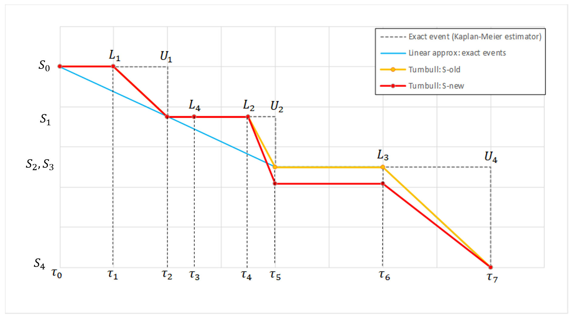
- The difference between the blue curve and \(S^{old}\) comes from the fact that \(S^{old}\) is interpolated on a grid including the \(L_i\) time points while they are not included in the grid considered in the case of exact events.
- The first iteration of the Turnbull agorithm has the effect of lowering \(S^{new} \)compared to \(S^{old}\) after \(\tau_4\), which is due to the fact that the event in \((L_4,U_4]\) may have already occured after that point.
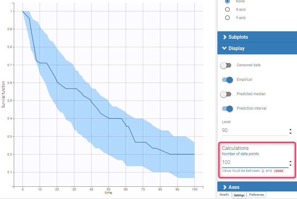
3. Prediction interval
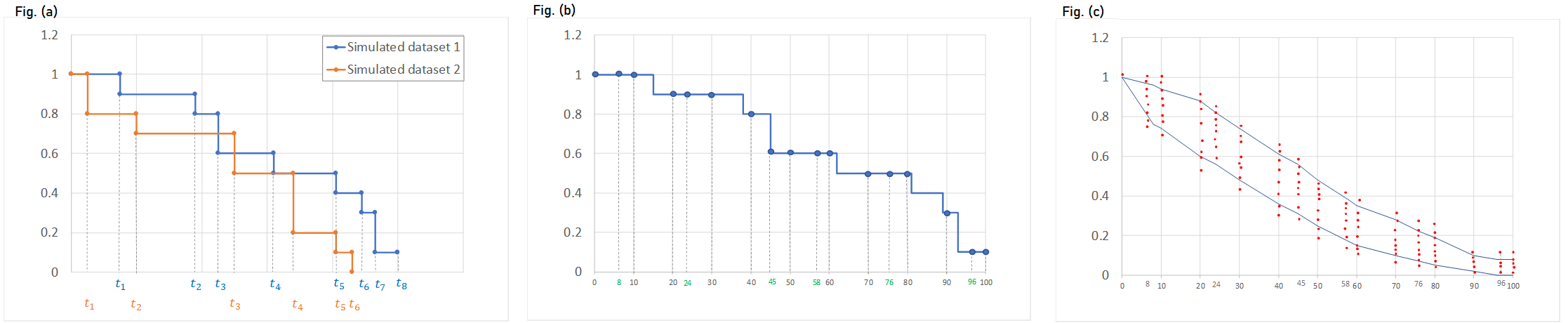
To generate the prediction interval in the VPC plot, Monolix performs by default 500 simulations with N individuals as in the original data set. As a result, it produces 500 time series that form 500 survival curves (based on Kaplan-Meier or Turnbull estimators). Since simulated event times are random numbers, all estimated survival functions have different time grids.This is shown on Fig.(a) with two different simulated datasets.
The interpolation of these curves on a fixed time grid allows to calculate the prediction interval. In Monolix the default time grid consists of a uniform grid with 100 points. For exactly observed events, the grid includes in addition all time points from the original data set to provide all possible information. Exact event times are unknown for interval censored events, so dataset time points have no additional information. This is shown on Fig.(b) with the Kaplan-Meier plot from the simulated dataset 1 from Fig.(a), interpolated on a different time grid than its events, combining regularly spaced points at times 0, 10, 20, …, 100, and additional time points indicated in green that come from the original dataset.).
The interpolation on the new grid gives at each time point of the grid a set of probabilities corresponding to different simulated survival curves. It allows to calculate lower and upper percentiles (the 5th and 95 percentiles are the default choice) and draw the prediction interval. This is shown on Fig.(c) with the survival estimators from multiple simulations on the same time grid as on Fig. (b).
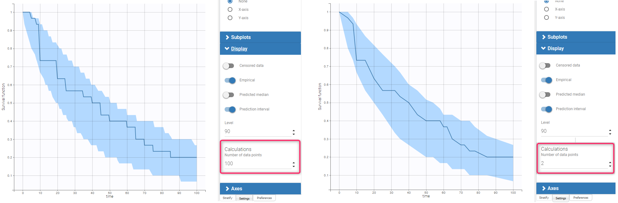
Example 1: exactly observed events
The dataset contains times of exactly observed single events of 30 individuals. The survival model has a constant hazard function and the Kaplan-Meier estimator approximates the survival function. The VPC plot uses a linear approximation of the Kaplan-Meier curve (Fig. on the left). By default, the fixed grid has 100 uniformly distributed points together with all time points from the date set. The figure on the left presents the VPC plot with the default settings. The approximation of the empirical and simulated Kaplan-Meier curves is sufficient on the default grid. In contrast, the VPC on the Figure on the right uses a grid with only time points from the original dataset. The accuracy of the prediction interval is decreased.
Example 2: interval censored events
In this dataset, the times of events from the previous example are the ends of time intervals within which events occurred. The length of the censored intervals in the dataset is non constant among individuals, and oscillates around 5. The structural model includes this information in eventTime and intervalLength options.