It is always good to have a look first at the observed data before running the parameter estimation. Indeed, it is very convenient to see if all the data is consistent, or if some outliers appear. Moreover, looking at the plot can help to identify hypotheses about the model, such as covariate effects. Three types of data can be visualized in Monolix using the graphical interface: continuous data, dicrete data and time-to-event data.

• Continuous data
• Discrete data
• Time-to-event data
• Settings
• Troubleshooting

Continuous data

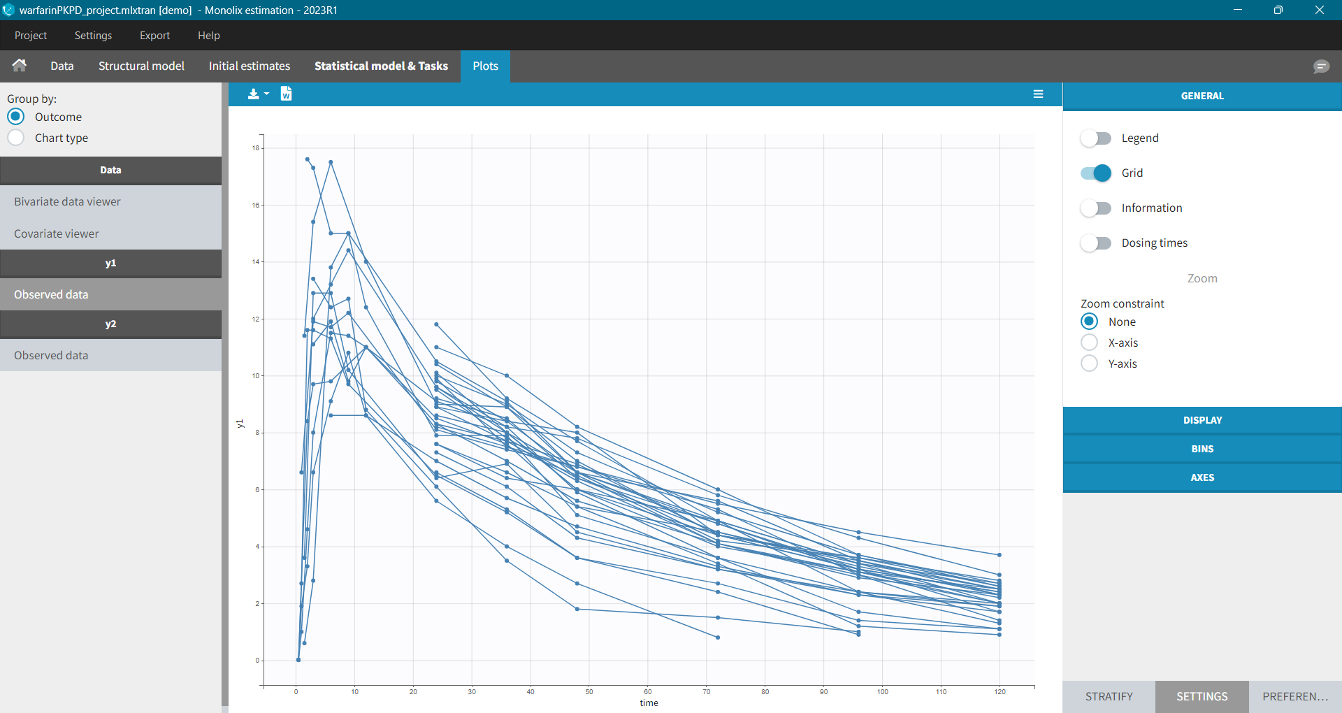
The purpose of this plot, also called a spaghetti plot, is to display the observed data (from a dataset loaded in Monolix) w.r.t. time. It is available in the PLOTS tab after loading and accepting a dataset in the DATA tab. You can access data for different observation in the left panel.

 

Settings in the right panel allow to adapt the plots display, full description is here.

General settings

General settings include: legend, display of grid, information about the data and dosing times.

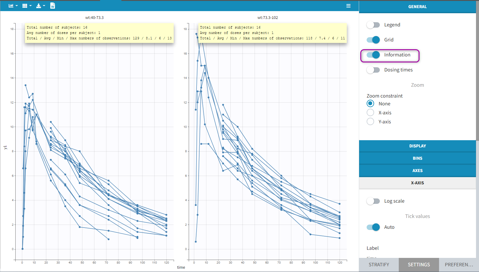
Information adds a box with summary of the data and is recomputed for each subplot after splitting by a covariate. It includes:

• The total number of subjects
• The average number of doses per subject
• The total, average, minimum and maximum number of observations per individual.

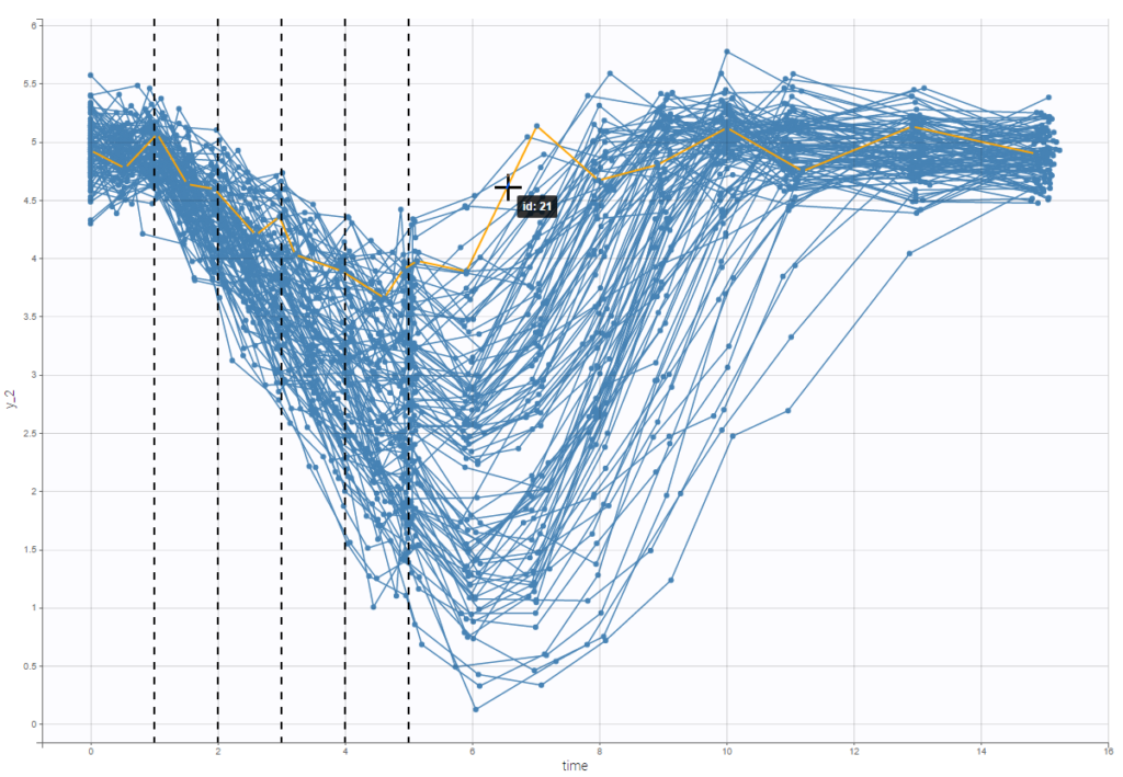
Option “dosing times” adds the individual dosing time as dashed vertical lines. You can make the lines always visible or only when you hover on individual data. Dosing times corresponding to doses with null amounts are not displayed.

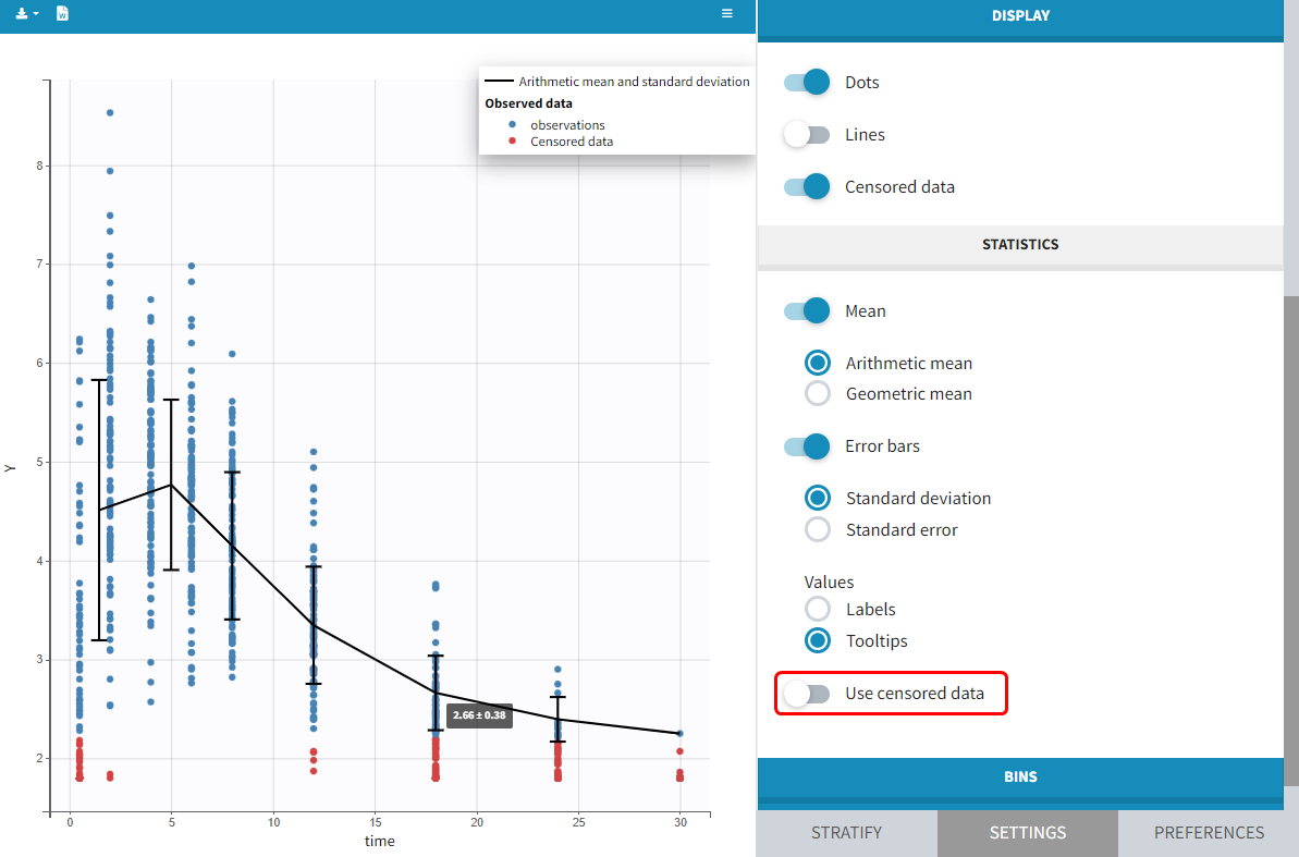
Display

You can display data as dots and lines (by default), or only as dots or only as lines, as in the figure below. Toggle “Mean” overlays a trend line on the plot, based on mean values of the observed data pooled in bins: arithmetic or geometric mean. Toggle “error bars” adds error bars as either the standard deviations or standard errors. The mean and error values can be displayed as fixed labels next to the bars, or as tooltips when hovering on a bar. If profiles contain censored data, these are by default displayed as red data points. Since version 2024, they can be hidden, if required, in the display section using the “Censored data” toggle. To avoid a possible distortion of the trend line, censored data can be excluded by disabling the “Use censored data” toggle in the statistics subsection

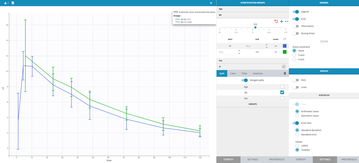
It is possible to display the mean curves, split by covariate, in a single plot. After split by a covariate, switch on the “Merged splits” option.  In the example below, the mean curves of the two weight groups, which were in separate plots, are merged into a single plot. This feature is available for versions Monolix 2023 and above.

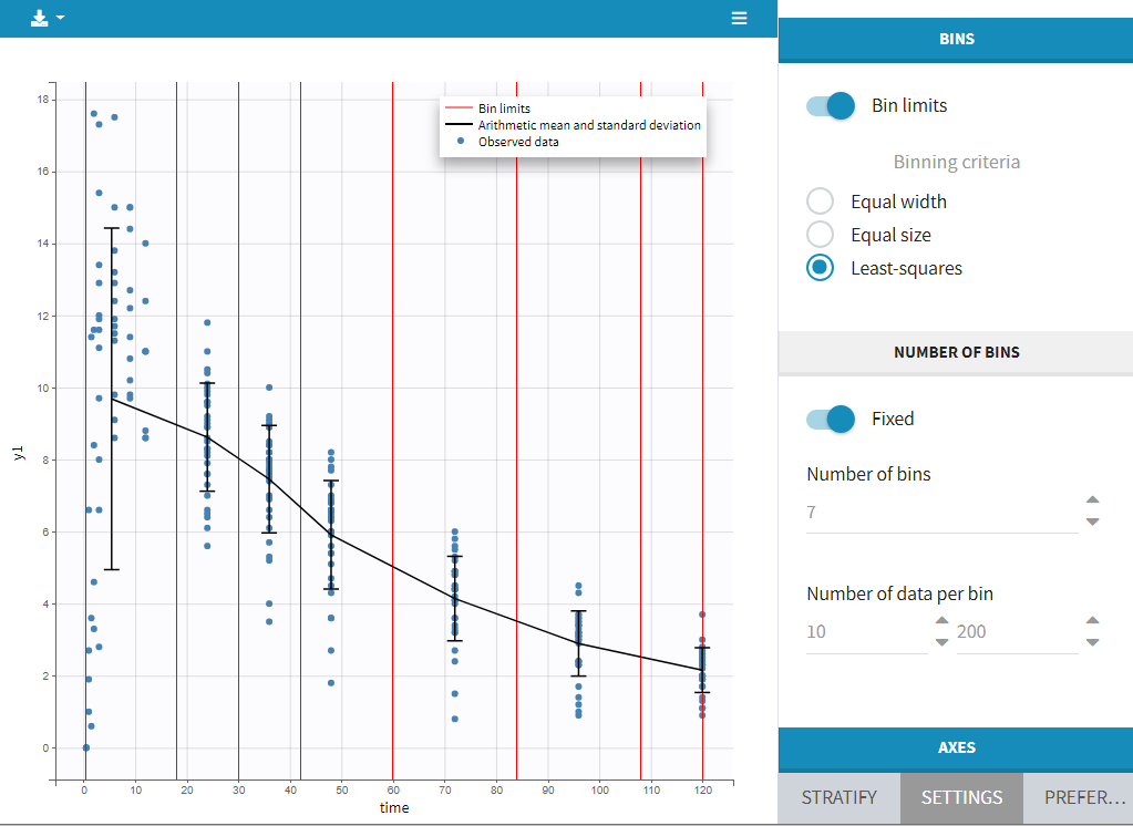
Bins

This section contains settings related to the definition of bins used in the computation of plot statistics. Toggle “bin limits” add vertical lines corresponding to the limits. In this section you can change the number of bins as well as binning criteria.

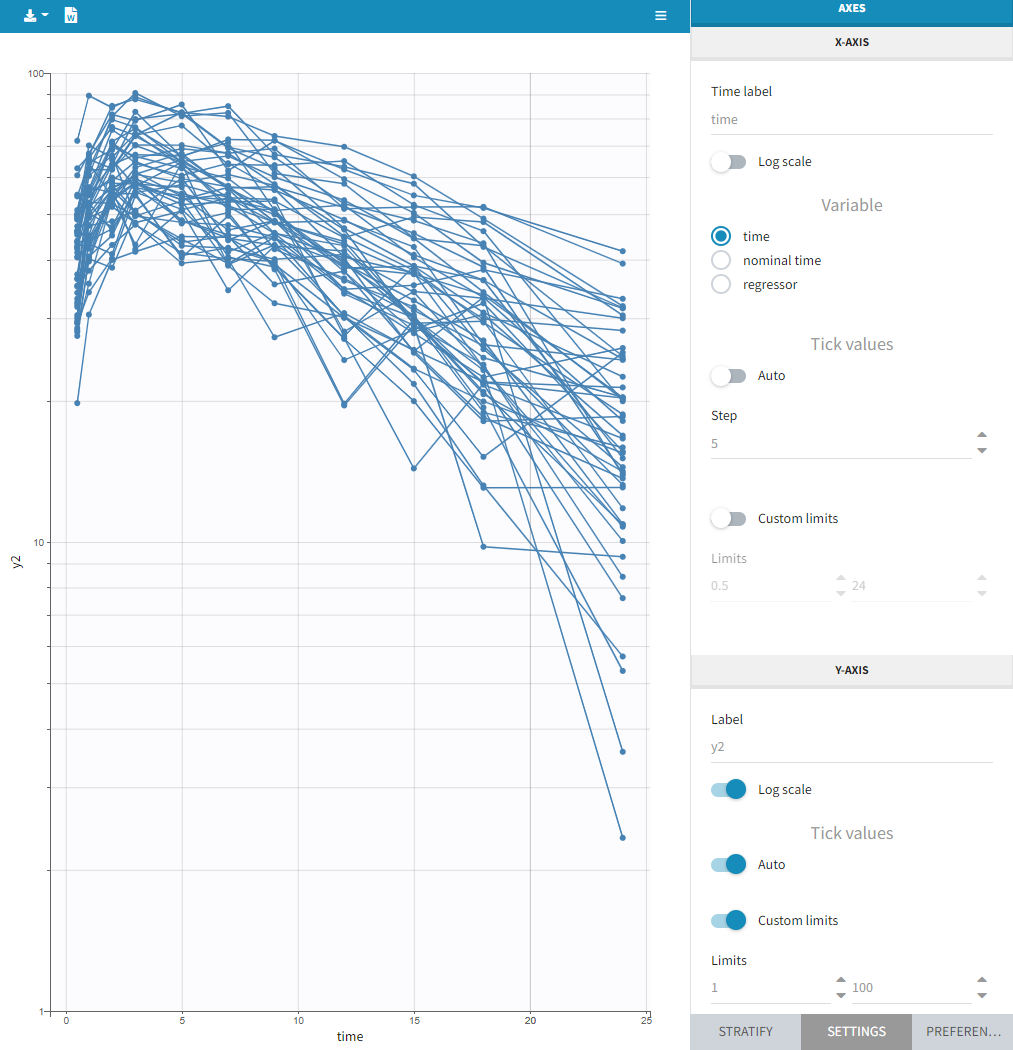
Axes

This section contains settings related to the display of X and Y – axis.

• Log scale toggle applies logarithm on a selected axis, for example to have a better evaluation of the elimination part.
• Nominal time option allows the nominal time to be displayed as time axis. This option is only available if nominal time has been tagged as such in the dataset (available in version 2024 and higher)
• Regressor option allows the values of the regressors tagged in the dataset to be displayed as x-axis (available in version 2024 and higher)
• Tick values “Auto” applies automatic axis ticks – if the toggle is enabled – or with a custom step – if the toggle is disabled.
• Label is an editable text displayed on each axis.
• Custom limits, when enabled, allows to choose the axis limits manually. They are applied to all subplots obtained by splitting by covariates.

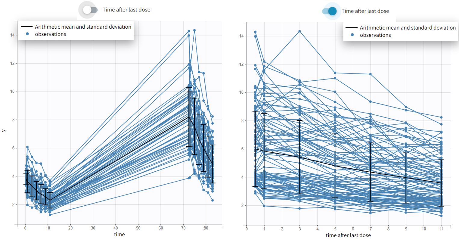
• Time after last dose toggle shows the spaghetti plot using on the x-axis time relative to the last dose (for Monolix version 2024 and higher). Below an example based on the demo project multidose_project.melxtran (Monolix demo folder 6.3)

Discrete data

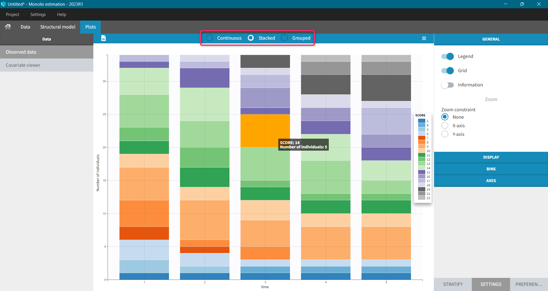
Monolix uses also count or categorical data, see here for detailed examples. Observed data can be shown as continuous, stacked or grouped. Example below shows the evolution of scores, which are categories describing anxious disorders, from the zylkene-data-set. The x-axis is time of measurements, while y-axis shows number of individuals in each category (different colors) at each time point. You can display the number of individuals for each category by hovering on it in the plot.

Settings, stratification and preferences work as for continuous data.

Time-to-event data

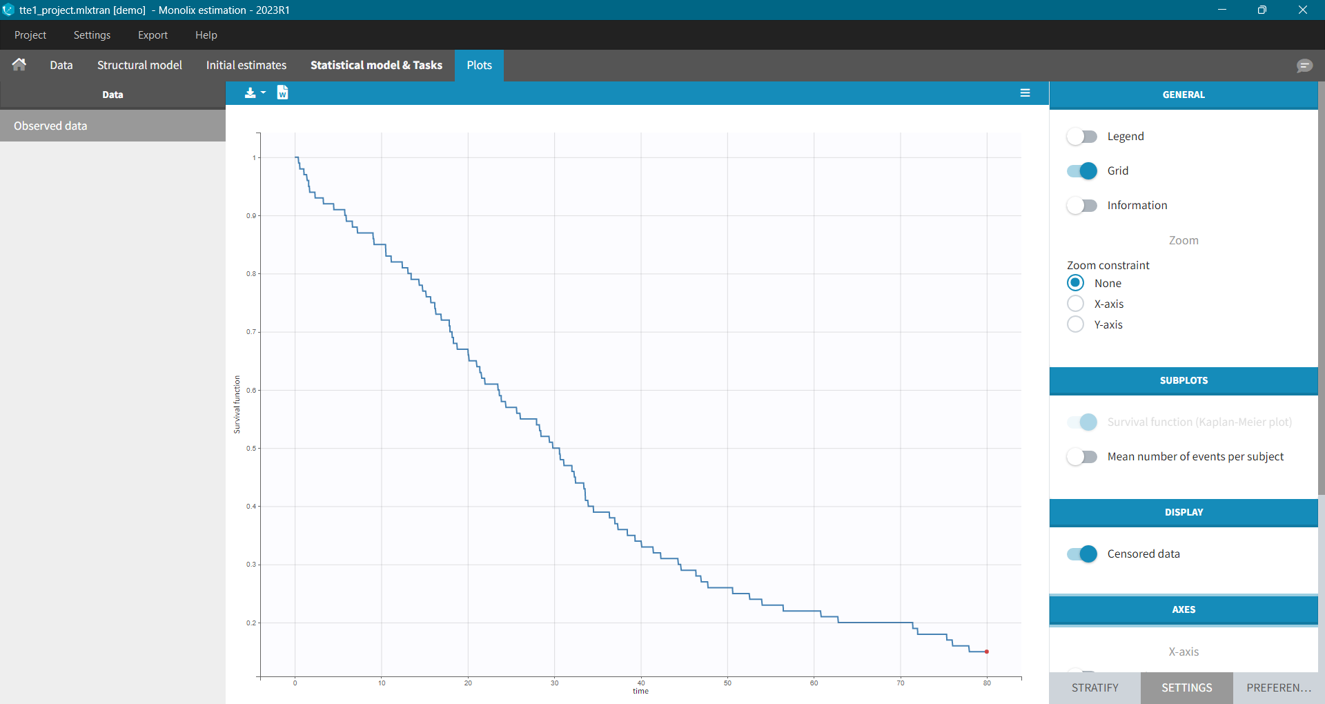
In Monolix, time-to-event data is displayed via a survival function, which describes the probability that an event happens after some time t. In general, this function is unknown and Monolix uses the non-parametric Kaplan-Meier estimator. It describes the probability that an individual survives until time t, knowing that it survived at any earlier time.

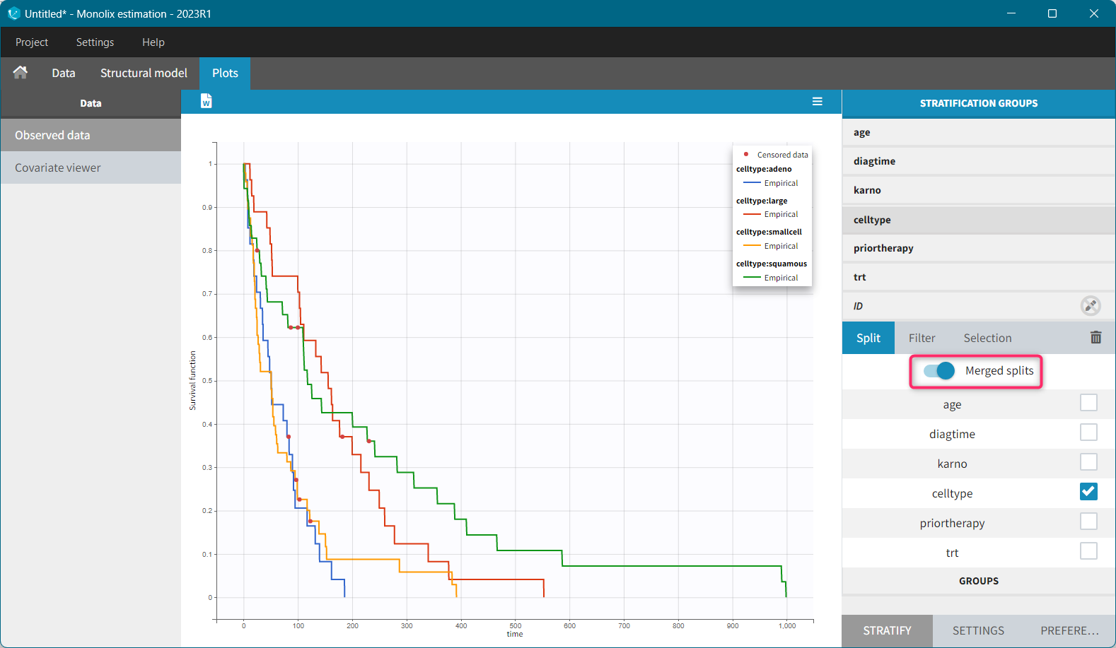
 It is possible to display the Kaplan – Meier plot split by covariate in a single plot. After split by a covariate in the Stratify sub-tab, switch on the “Merged splits” option. In the example below, the curves of the four cell type groups, which were in separate plots, are merged into a single plot.

Kaplan – Meier estimator

For a single event data, the Kaplan-Meier estimator is given by the following formula
\( \hat{S}(t)=\sum_{i:t_i<t} \left(1-d_i/n_i\right),\)
where

• (t_i) – times before t, when at least one event occurred,
• (d_i) – number of events at the time (t_i),
• (n_i) – number of individuals at risk, that is who did not experience an event until (t_i).

The probability that an event occurs ((p_e)) is the ratio between the number of events that has occurred ((d_i)) and the total number of individuals at risk ((n_i)). The complement of it, ((1-p_e)), gives an estimation of the survival. For each time t the total number of individuals at risk changes, so the probabilities at all previous times (t_i), when at least one event occurred, are multiplied. It is similar to calculating the probability that a patient survives 2 days. It is a product of a probability that a patient survives the first day and a conditional probability that it survives the second day, knowing that it survived the first one.

Example:

A typical example of a time-to-event data set contains information about exact times when individuals experienced an event or when they left a study (drop-out). In the following, there are five individuals, who have two observations: time when the observation starts, which is 0 for all, and time of an event. If a patient leaves a study, then the time of a drop-out is given but instead of 1 in the column for the observation, there is 0. It indicates that this individual didn’t experience an event but survived until the drop-out time.The advantage of the Kaplan-Meier estimate is that it takes into account situations when not all individuals continue the study. At the next event time, such individuals are not counted as individuals at risk (they are not counted in the denominator (n_i)).

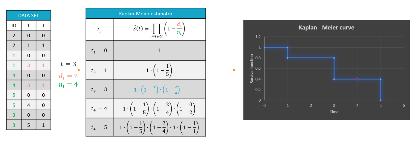
A study starts at time (t_1). There are no events, so (d_1=0) and the value of the survival curve is 1. Until the next event time at (t_2=1), the survival remains constant. Then, one individual experienced an event, so (d_2=1), and all individuals survived until that time, so (n_2=5). The result is that the probability to survive decreases by 0.2, which corresponds to the height of the jump at (t=1) in the plot. Then again, until the next event, survival remains constant. At time (t=3), there are two events. The number (n_3) counts now only 4 individuals – it has decreased by 1 due to the previous event. To get the final value probability at time 3is multiplied by all earlier probabilities. At (t=4) there is a drop-out. Patient 5 left the study and no event was registered. The survival curve remains constant, and the drop-out is marked in red. The Kaplan-Meier estimator takes into account this situations, because at the next event time (t=5), this individual is not counted as an individual at risk – denominator n will be smaller. At time (t=5), there is only one individual left, and one event, so the survival equals 0.

Remarks

• Kaplan-Meier estimator handles correctly information about individuals who left the study, but there is a bias when the exact times of events are unknown.
• In data visualization, Monolix assumes that all events are exactly observed. For example: assume that an observation period started at (t=0) and at (t=1) an event is marked by 1 in the column for the observation. It is impossible to distinguish in the dataset, without any other information, if the event was exactly at (t=1) or before. The same problem is when a time of the beginning of the study and time interval limits of an event are given. Just looking at the data set, an exact and interval censored event type are indistinguishable. In other words, not knowing when an event happened, Monolix assumes that it happened at the end of the censored interval.

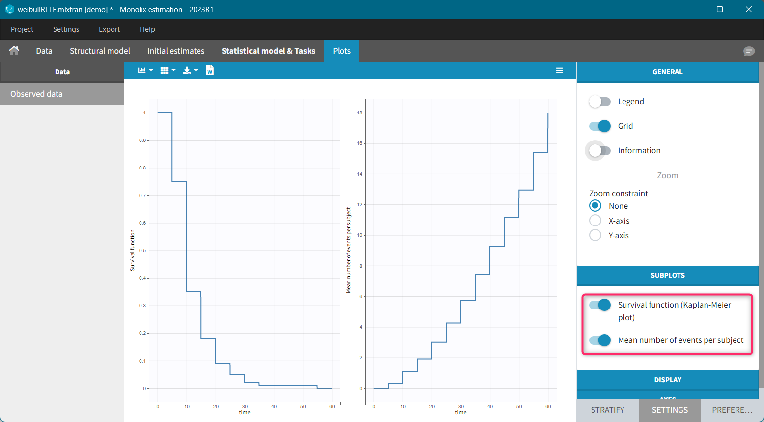
Mean number of events.

The Kaplan-Meier estimator can be used also for the analysis of repeated events. The survival curve is estimated for each k-th event separately ( \hat{S}^{(k)}(t) = \sum_{i:t_i<t} \left(1-\frac{d^{(k)}i}{n^{(k)}_i}\right)), and is used to calculate the mean number of events per individual as a function of time (\hat{m}(t) = \sum{k} \left(1-\hat{S}^{(k)}(t)\right).) It can be visualized next to the Survival function by choosing this option from the Subplots settings:

 

Settings

• General: Add/remove the legend, the grid, data information and dosing times; constrains on zoom
• Display: add/remove data dots, lines, mean and error bars
• Bins: display bin limits, binning criteria, number of bins
• Axes: Add/remove log-scale, modify labels, set tick values, set custom axis limits
• Stratify: Split, color and filter by covariates,
• Preferences: Add/remove elements or change colors and sizes for axes, observations, censored (BLQ) observations, highlighting.