- Interacting with the plots
- Highlight: tooltips and ID
- Stratification: split, color, filter
- Layout
- Preferences: customizing the plot appearance
Interactive diagnostic plots
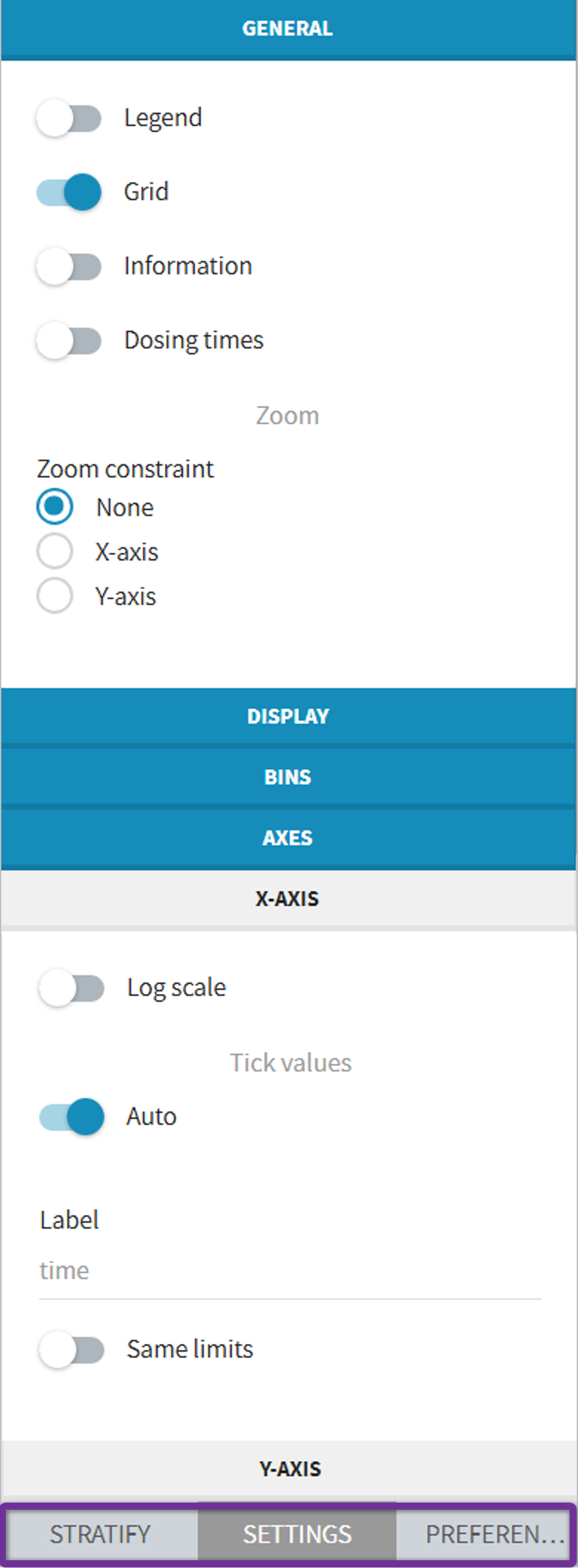
In the PLOTS tab, the right panel has several sub – tabs (at the bottom) to interact with the plots:
- The tab “Settings” provides options specific to each plot, such as hiding or displaying elements of the plot, modifying some elements, or changing axes scales, ticks and limits.
- The tab “Stratify” can be used to select one or several covariates for splitting, filtering or coloring the points of the plot. See below for more details.
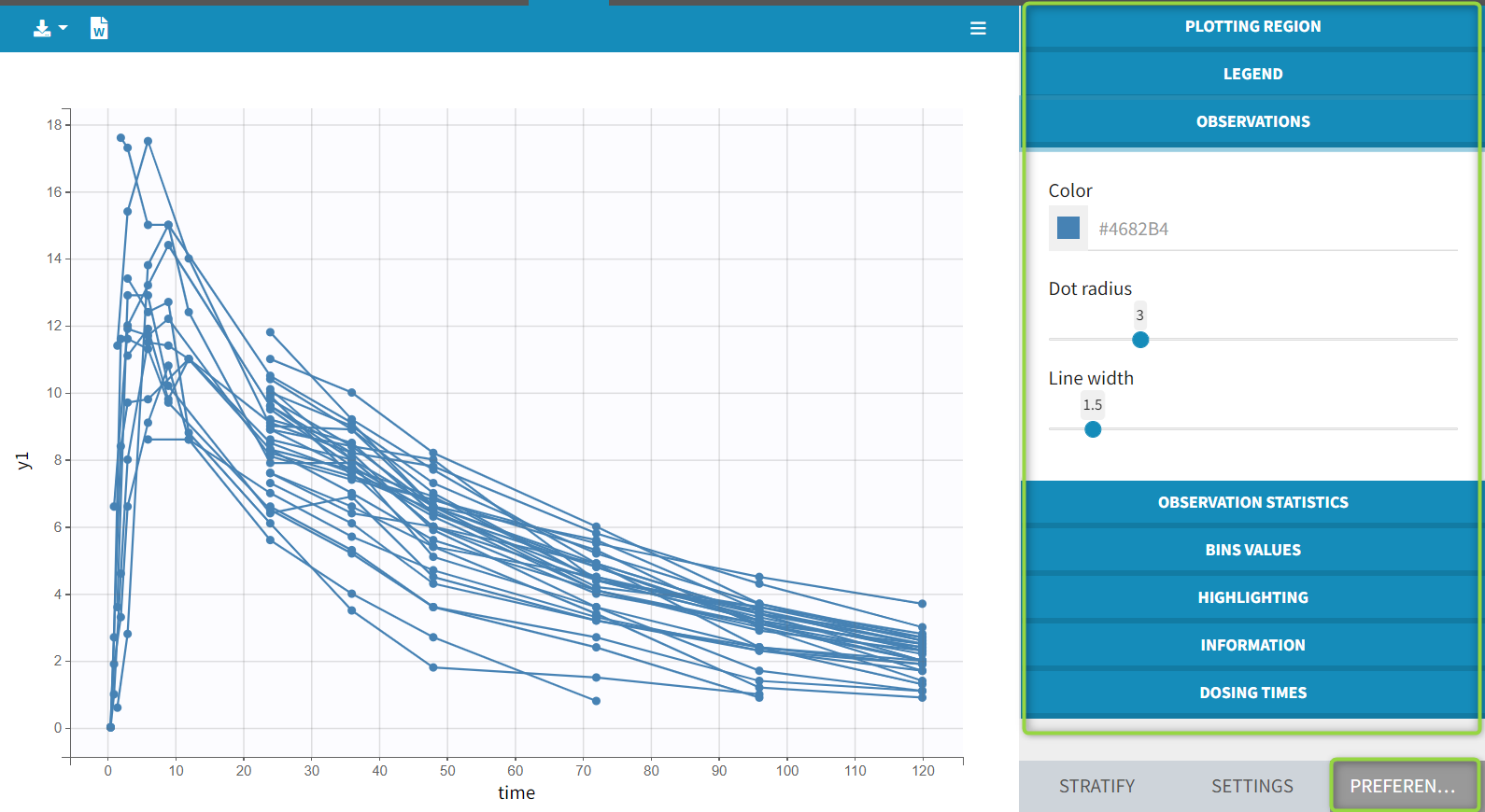
- The tab “Preferences” alows to customize graphical aspects such as colors, font size, dot radius, line width, …
These tabs are marked in purple on the following figure, which is the panel that is showed for observed data:
Highlight: tooltips and ID
In all the plots, when you hover a point or a curve with your mouse, some informations are provided as tooltips. For example, the ID is displayed when hovering a point or the curve of an individual in the observed data plot, the ID, the time and/or the prediction is displayed in the scatter plot of the residuals.
In addition, starting from the 2019 version, when hovering one point/ID in a plot, the same ID will be highlighted in all the plots with the same color.
Stratification: split, color, filter
The stratification panel allows to create and use covariates for stratification purposes. It is possible to select one or several covariates for splitting, filtering or coloring the data set or the diagnosis plots as exposed on the following video.
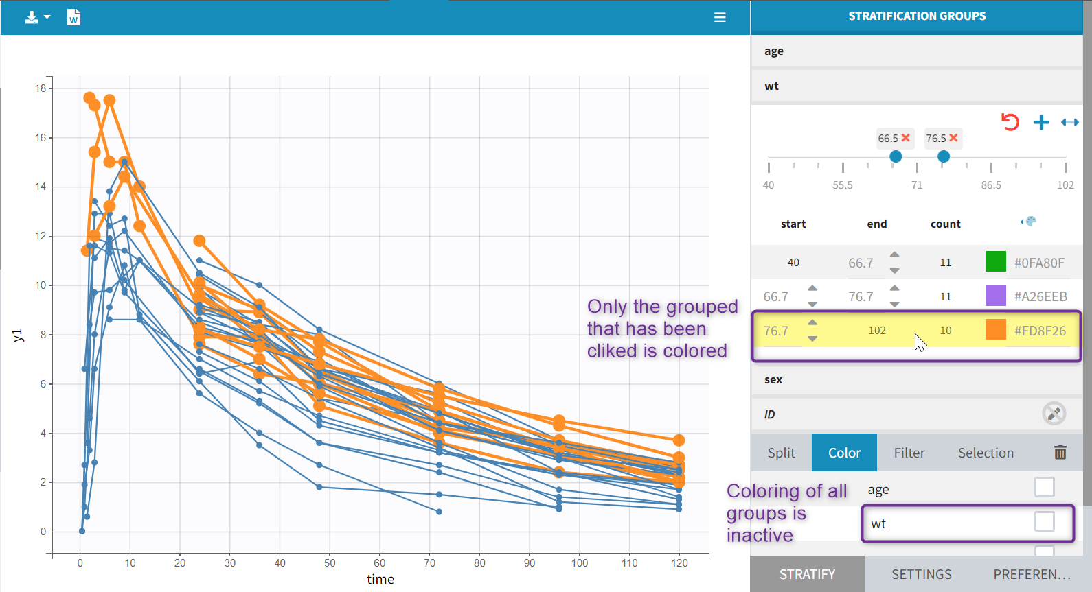
The following figure shows a plot of the observed data from the warfarin dataset, stratified by coloring individuals according to the continuous covariate wt: the observed data is divided into three groups, which were set to equal size with the button “rescale”. It is also possible to set groups of equal width, or to personalize dividing values.
In addition, the bounds of the continuous covariate groups can be changed manually.
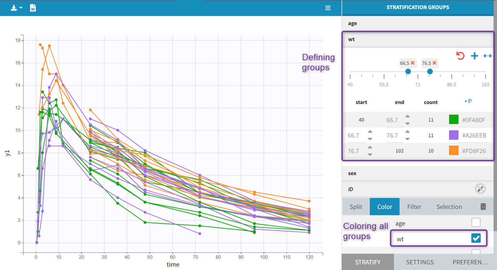 Moreover, clicking on a group highlights only the individuals belonging to this group, as can be seen below:
Values of categorical covariates can also be assigned to new groups, which can then be used for stratification.
In addition, the number of subjects in each categorical covariate groups is displayed.
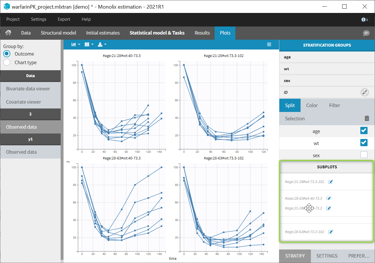
Starting from the 2021R1 version, the list of subplots obtained by split is displayed below the split selection. It is possible to reorder the items in this list with drag-and-drop, which also reorders the subplot layout. Moreover, an “edit” icon next to each subplot name in the list allows to change the subplot titles.
Preferences: customizing the plot appearance
In the “preferences” tab, the user can modify the different aspects of the plot: colors, line style and width, fonts and label position offsets, …
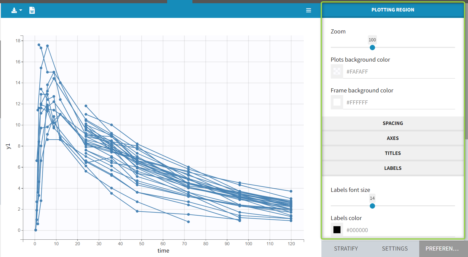
The following figures show on the warfarin demo the choices for the plot content and the choices for the labels and titles (in the “Plotting region” section). The sizes of all elements of the plots can also be changed with the single “zoom” preference in “Plotting region”.
Layout
The layout can be modified with buttons on top of each plot.
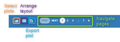
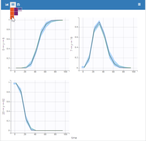
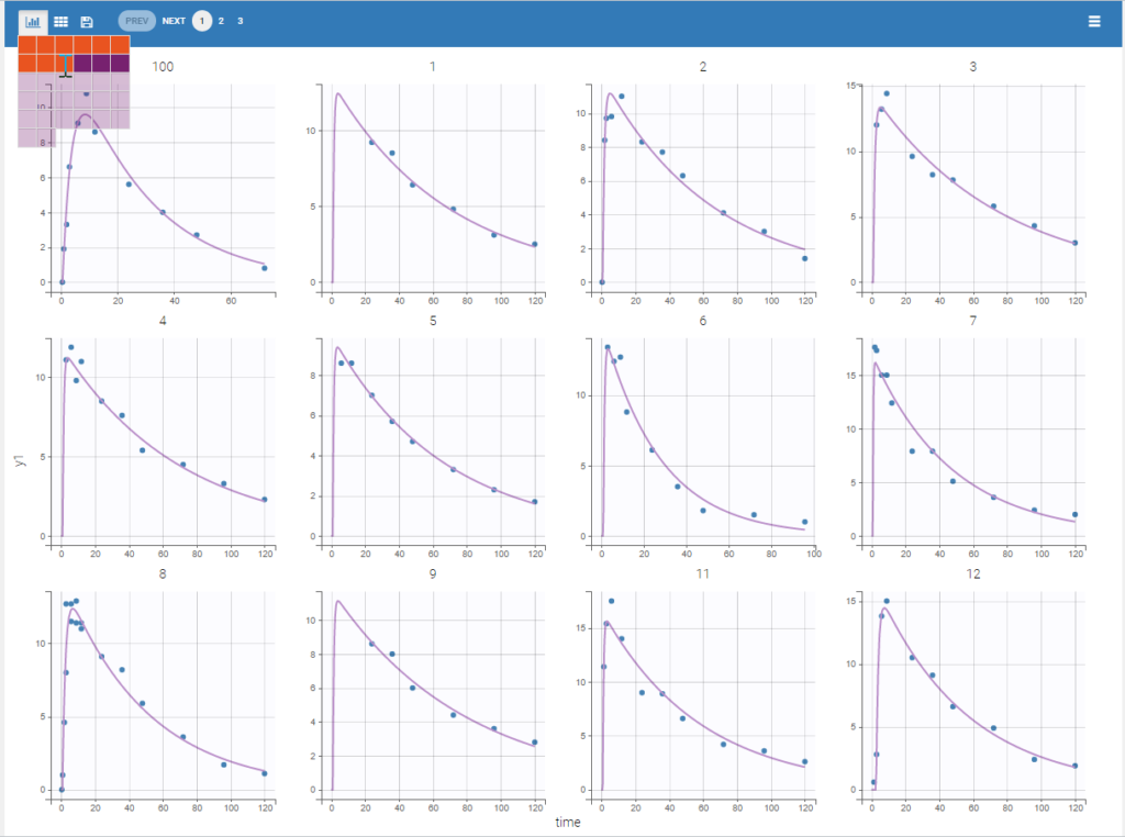
The first button can be used to select a set of subplots to display in the page. For example, as shown below, it is possible to display 9 individual fits per page instead of 12 (default number). The layout is then automatically adapted to balance the number of rows and columns.
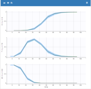
The second button can be used to choose a custom layout (number of rows and columns). On the example figures below, the default layout with 3 subplots (left) is modified to arrange them on a single column (right).