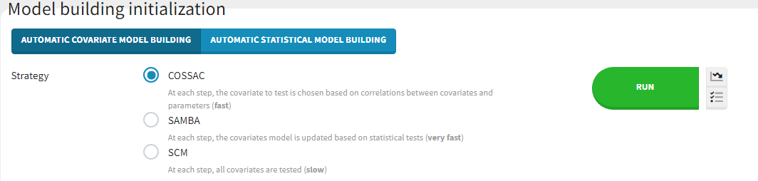
Starting from the 2019 version, automatic covariate model building algorithms are implemented in Monolix, and can be chosen in the “Initialization” tab of the Model building panel:
SCM
This is the classic stepwise covariate modeling method. A set of iterations of forward selection is followed by a set of iterations of backward selection.
In the forward selection, at each step, each of the remaining (i.e not yet included) parameter-covariate relationships are added to the model in an univariate model (one model per relationship), and run. Among all models, the model that improves some criteria (LRT, or BICc) most is selected and taken forward to the next step. During backward elimination, parameter-covariate relationships are removed in an univariate manner.
This method is effective but expensive in terms of number of runs, because it requires to estimate the population parameters with SAEM and simulate individual parameters from Conditional distributions for each evaluated model.
COSSAC
COSSAC (COnditional Sampling use for Stepwise Approach based on Correlation tests) is a fast, innovative covariate search strategy that Lixoft validated and published here:
COSSAC makes use of the information contained in the base model run to choose which covariate to try first (instead of trying all covariates “blindly” as in SCM). Indeed, the correlation between the individual parameters (or random effects) and the covariates hints at possibly relevant parameter-covariate relationships. If the EBEs (empirical Bayes estimates) are used, shrinkage may bias the result. COSSAC instead uses samples from the a posteriori conditional distribution (available as “conditional distribution” task in Monolix) to calculate the correlation between the random effects and covariates. A p-value can be derived using the Pearson’s correlation test for continuous covariate and ANOVA for categorical covariate. The p-values are used to sort all the random effect-covariate relationships, whether they are included in the model or not.
The iterations of COSSAC alternate between a forward selection and a backward selection, depending on the results of the correlation tests:
- Initialization:
- Run the base model (population parameter estimation, conditional distribution sampling, and log-likelihood estimation).
- Calculate the p-values of all the parameter-covariate relationships using Pearson’s correlation tests and ANOVA (automatically done in Monolix)
- Start with a backward selection.
- Forward selection:
- Add the covariate with the smallest correlation p-value (among the remaining parameter-covariate relationships) to the model, or the next smallest if the smallest has already been tried, and so until no correlation p-values above a threshold remain
- Run the model with the same initial values as the base model (initial estimates for the new beta parameters are 0)
- Accept/reject the relationship based on the likelihood ratio test or BICc: the model is not retained if the criteria does not improve (with a threshold for the likelihood ratio test)
- Calculate all parameter-covariate correlation p-values
- Try a backward selection
- Backward selection:
- Among the covariates present in the model, remove the covariate with the highest (less significant) correlation p-value, or the next highest if the highest has already been tried, and so until no correlation p-values below a threshold remain
- Run the model with the same initial values as the base model (initial estimates for the new beta parameters are 0)
- Accept/reject the relationship removal based on the likelihood ratio test or BICc: the model is not retained if the criteria does not improve (with a threshold for the likelihood ratio test)
- Calculate all parameter-covariate relationship correlation p-value
- Try a forward selection
- The algorithm continues until no forward or backward selection is possible, or after testing 10 new relationships on the same model.
- Relationships between covariates and parameters without variability can not be explored with COSSAC, therefore parameters without variability are handled with SCM at the end of COSSAC.
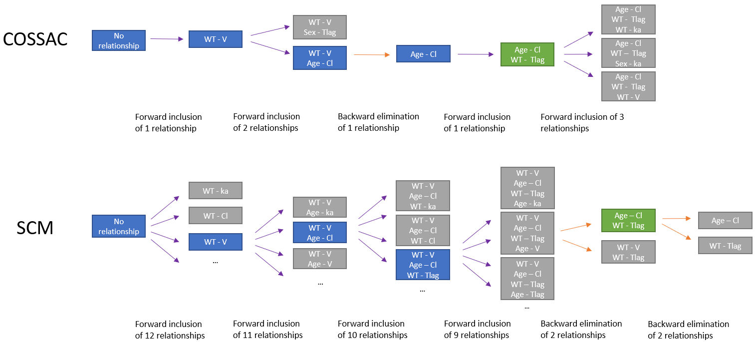
Example
The major difference between SCM and COSSAC is that very few iterations are usually needed with COSSAC before deciding to add or remove a parameter-covariate relationship: between 1 and 10, depending on the number of significant correlations and the improvement brought by each new relationship.
The schema below illustrates this difference on an example with 4 parameters (ka, V, Cl, Tlag) and 3 covariates (Age, Sex, WT). Purple arrows represent forward selections while orange arrows represent backward selections. Starting from a model with no relationship between parameters and covariates, each model run in a new iteration is represented with a rectangle, colored in blue if the model is kept as a starting point for the next iteration, or in grey if the model does not bring improvement. Final models are colored in green. In the case of COSSAC, 1 iteration is sufficient to update the model except at the second step, because the first relationship tried (Sex on eta_Tlag) does not improve the criteria. At the last step only 3 relationships with a remaining p-value below the threshold have to be tested before finishing. In the case of SCM, all models run are not displayed but the number of iterations at each step is written. In total, 45 models are run during the SCM procedure, while COSSAC needs only 8 models.
SAMBA
Starting from the 2021 version, with “SAMBA” in the covariate model building panel, it is possible to run SAMBA algorithm applied only to the covariate effects. At each iteration, the model is run, the Proposal is calculated and applied (taking into account only the covariates and not the error model or correlations) and this new model is then run in the next iteration. The algorithm stops when the Proposal does not suggest any change any more (or if an already tested model is suggested by the proposal).
At each iteration, several covariates can be added or removed, thus SAMBA is very fast.
Settings
The linearization method is selected by default to compute the log-likelihood of the estimated model at each iteration. It can be unselected to use importance sampling.
The improvement can be evaluated with two different criteria based on the log-likelihood, that can be selected in the settings (available via the icon next to Run):
- BICc (by default)
- LRT (likelihood ratio threshold): by default the forward threshold is 0.01 for COSSAC and 0.05 for SCM, and the backward threshold is 0.01. These values can be changed in the settings.
By default, the correlation thresholds to add new covariate effects in COSSAC (forward) is 0.5 and the correlation threshold to remove some covariate effects in COSSACc(backward) is 0.01. These values can be changed in the settings.
Starting from the 2021 version, all settings used are saved and reloaded with the run containing the model building results.
The estimation tasks for all runs are set automatically to “population parameter”, “EBEs”, “conditional distribution” and “likelihood”, independently of the tasks selected in the base (parent) run.
Selecting covariates and parameters
It is possible to select part of the covariates and individual parameters to be used in the algorithm:

Moreover, a panel “Locked relationships” can be opened to lock in or lock out some covariate-parameter relationships among the ones that are available:
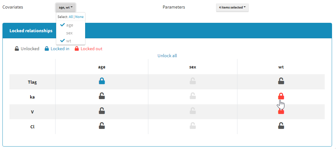
Starting from the 2021 version, all relationships considered in model building are part of the settings which are saved and reloaded with the run containing the model building results.
Results
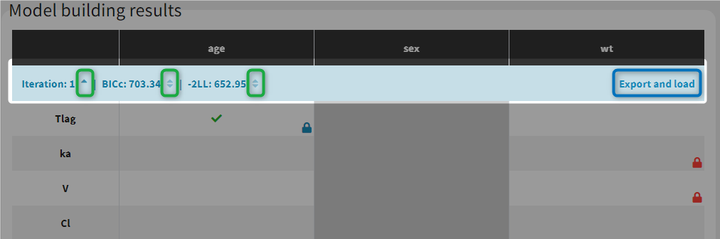
The results of the model building are displayed in a tab Results, with the list of model run at each iteration (see for example the figure below). All resulting runs are also located in the ModelBuilding subfolder of the project’s result folder (located by default next to the .mlxtran project file).
In the Results tab, by default runs are displayed by order of iteration, except the best model which is displayed in first position, highlighted in green. Differences with the previous iteration are highlighted in yellow. Parameters or covariates that have been excluded from the covariate search appear in grey. Locked in or locked out relationships are also indicated with a blue or red icon.
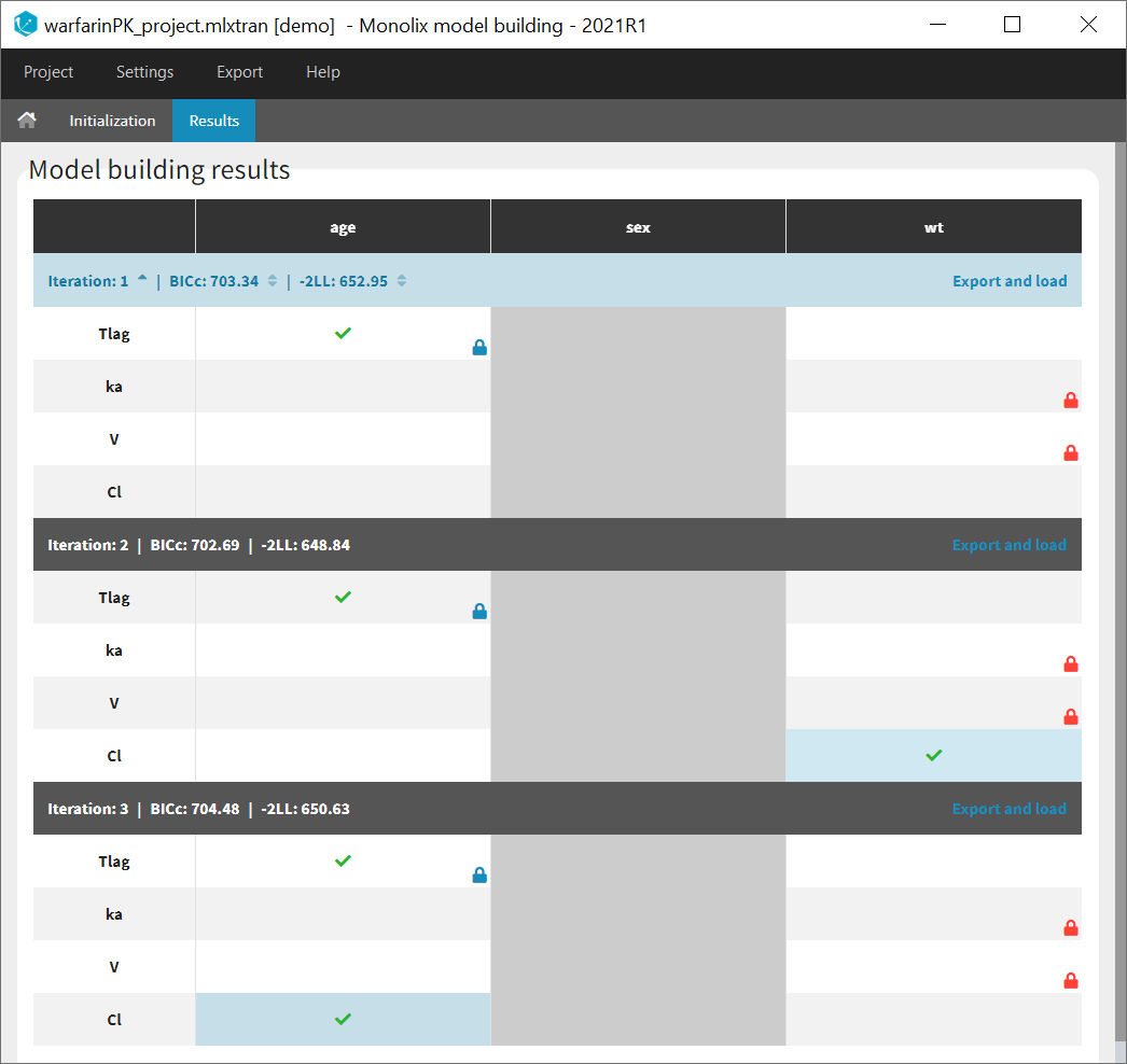
Note that the table of iterations can be sorted by iteration number or criteria (see green marks below). Buttons “export and load” (see blue mark below) can also be used to export the model estimated at this iteration as a new Monolix project with a new name.