- Purpose
- Calculation of the conditional distribution
- Conditional distribution
- MCMC algorithm
- Conditional mean
- Samples from the conditional distribution
- Stopping criteria
- Running the conditional distribution estimation task
- Outputs
- In the graphical user interface
- In the output folder
- Settings
Purpose
The conditional distribution represents the uncertainty of the individual parameter values. The conditional distribution estimation task permits to sample from this distribution. The samples are used to calculate the condition mean, or directly as estimators of the individual parameters in the plots to improve their informativeness [1]. They are also used to compute the statistical tests.
Calculation of the conditional distribution
Conditional distribution
The conditional distribution is \(p(\psi_i|y_i;\hat{\theta})\) with \(\psi_i\) the individual parameters for individual i, \(\hat{\theta}\) the estimated population parameters, and \(y_i\) the data (observations) for individual i. The conditional distribution represents the uncertainty of the individual’s parameter value, taking into account the information at hand for this individual:
- the observed data for that individual,
- the covariate values for that individual,
- and the fact that the individual belongs to the population for which we have already estimated the typical parameter value (fixed effects) and the variability (standard deviation of the random effects).
It is not possible to directly calculate the probability for a given \(\psi_i\) (no closed form), but is possible to obtain samples from the distribution using a Markov-Chain Monte-Carlo procedure (MCMC).
MCMC algorithm
MCMC methods are a class of algorithms for sampling from probability distributions for which direct sampling is difficult. They consist of constructing a stochastic procedure which, in its stationary state, yields draws from the probability distribution of interest. Among the MCMC class, we use the Metropolis-Hastings (MH) algorithm, which has the property of being able to sample probability distributions which can be computed up to a constant. This is the case for our conditional distribution, which can be rewritten as:
$$p(\psi_i|y_i)=\frac{p(y_i|\psi_i)p(\psi_i)}{p(y_i)}$$
\(p(y_i|\psi_i)\) is the conditional density function of the data when knowing the individual parameter values and can be computed (closed form solution). \(p(\psi_i)\) is the density function for the individual parameters and can also be computed. The likelihood \(p(y_i)\) has no closed form solution but it is constant.
In brief, the MH algorithm works in the following way: at each iteration k, a new individual parameter value is drawn from a proposal distribution for each individual. The new value is accepted with a probability that depends on \(p(\psi_i)\) and \(p(y_i|\psi_i)\). After a transition period, the algorithm reaches a stationary state where the accepted values follow the conditional distribution probability \(p(\psi_i|y_i)\). For the proposal distribution, three different distributions are used in turn with a (2,2,2) pattern (setting “Number of iterations of kernel 1/2/3” in Settings > Project Settings): the population distribution, a unidimensional Gaussian random walk, or a multidimensional Gaussian random walk. For the random walks, the variance of the Gaussian is automatically adapted to reach an optimal acceptance ratio (“target acceptance ratio” setting in Settings > Project Settings).
Conditional mean
The draws from the conditional distribution generated by the MCMC algorithm can be used to estimate any summary statistics of the distribution (mean, standard deviation, quantiles, etc). In particular we calculate the conditional mean by averaging over all draws:
$$ \hat{\psi}_i^{mean} = \frac{1}{K}\sum_{k=1}^{K}\psi_i^{k}$$
The standard deviation of the conditional distribution is also calculated. The number of samples used to calculate the mean and standard deviation corresponds to the number of chains times the total number of iterations of the conditional distribution task (not only during the convergence interval length). The mean is calculated over the transformed individual parameters (in the gaussian space), and back-transformed to the non-gaussian space.
Samples from the conditional distribution
Among all samples from the conditional distribution, a small number (between 1 and 10, see “Simulated parameters per individual” setting) is kept to be used in the plots. These samples are unbiased estimators and they present the advantage of not being affected by shrinkage, as shown for example on the documentation of the plot “distribution of the individual parameters“.
Stopping criteria
At iteration k, the conditional mean is calculated for each individual by averaging over all k previous iterations. The average conditional means over all individuals (noted E(X|y)), and the standard deviation of the conditional means over all individuals (noted sd(X|y)) are calculated and displayed in the pop-up window. The algorithm stops when, for all parameters, the average conditional means and standard deviations of the last 50 iterations (“Interval length” setting) do not deviate by more than 5% (2.5% in each direction, “relative interval” setting) from the average and standard deviation values at iteration k.
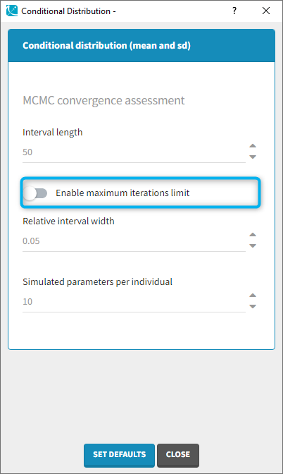
In some very specific cases (for example with a parameter with a normal distribution and a value very close to 1), it can take many iterations to reach the convergence criteria because the criteria is defined as a percentage. In that case, the toggle “enable maximum number of iterations” can be used to limit the number iterations of this task. If the limit is reached, a warning message will be displayed in the interface.
Running the conditional distribution estimation task
During the evaluation of the conditional distribution, the following plot pop-ups, displaying the average conditional means over all individuals (noted E(X|y)), and the standard deviation of the conditional means over all individuals (noted sd(X|y)) for each iteration of the MCMC algorithm.

The convergence criteria described above means that the blue line, which represents the average over all individuals of the conditional mean, must be within the tube. The tube is centered around the last value of the blue line and spans over 5% of that last value. The algorithm stops when all blue lines are in their tube.
Dependencies between tasks:
- The “Population parameters” task must be run before launching the conditional distribution task.
- The conditional distribution task is recommended before calculating the log-likelihood task without the linearization method (i.e log-likelihood via importance sampling).
- The conditional distribution task is necessary for the statistical tests.
- The samples generated during the conditional distribution task will be reused for the Standard errors task (without linearization).
Outputs
In the graphical user interface
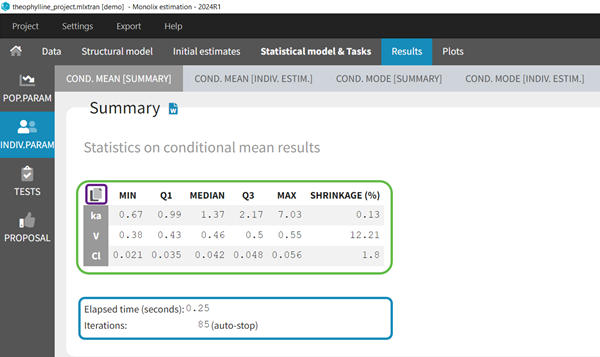
In the Indiv.Param section of the Results tab, a summary of the estimated conditional mean is given (min, max, quartiles, and shrinkage [in Monolix 2024 and later]), as shown in the figure below. Starting from Monolix2021R1, the number of iterations is also displayed, along with a message indicating whether convergence has been reached (“auto-stop”) or if the task was stopped by the user or reached the maximum number of iterations.
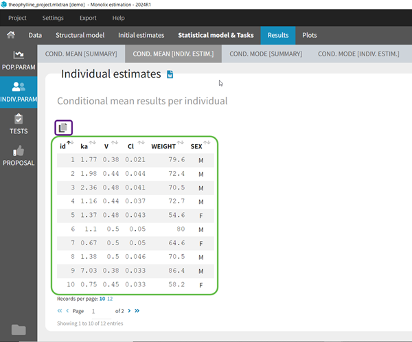
To see the estimated parameter value for each individual, the user can click on the [INDIV. ESTIM.] section. Notice that the user can also see them in the output files, which can be accessed via the folder icon at the bottom left. Notice that there is a “Copy table” icon on the top of each table to copy them in Excel, Word, … The table format and display will be kept.
In the output folder
After having run the conditional distribution task, the following files are available:
- summary.txt: contains the summary statistics (as displayed in the GUI)
- IndividualParameters/estimatedIndividualParameters.txt: the individual parameters for each subject-occasion are displayed. The conditional mean (*_mean) and the standard deviation (*_sd) of the conditional distribution are added to the file. The number of samples used to calculate the mean and standard deviation corresponds to the number of chains times the total number of iterations of the conditional distribution task (not only during the convergence interval length).
- IndividualParameters/estimatedRandomEffects.txt: the individual random effects for each subject-occasion are displayed. Those corresponding to the conditional mean (*_mean) are added to the file, together with the standard deviation (*_sd).
- IndividualParameters/simulatedIndividualParameters.txt: several simulated individual parameters (draws from the conditional distribution) are recorded for each individual. The rep column permits to distinguish the several simulated parameters for each individual.
- IndividualParameters/simulatedRandomEffects.txt: the random effects corresponding to the simulated individual parameters are recorded.
- IndividualParameters/shrinkage.txt: starting with Monolix 2024, the shrinkage for each parameter for the conditional mean as shrinkage_mean and for the conditional distribution as shrinkage_condDist.
More details about the content of the output files can be found here.
Settings
To change the settings, you can click on the settings button next the conditional distribution task.

- Interval length (default: 50): number of iterations over which the convergence criteria is checked.
- Relative interval (default: 0.05): size of the interval (relative to the current average or standard deviation) in which the last “interval length” iterations must be for the stopping criteria to be met. A value at 0.05 means that over the last “interval length” iterations, the value should not vary by more than 5% (2.5% in each direction).
- Simulated parameters per individual (default: via calculation): number of draws from the conditional distribution that will be used in the plots. The number is calculated as min(10, idealNb) with idealNb = max(500 / number of subject , 5000 / number of observations). This means that the maximum number is 10 (which is usually the case for small data sets). For large data sets, the number may be reduced, but the number of individual times the number of simulated parameters should be at least 500, and the number of observations times the number of simulated parameters should be at least 5000. This ensures to have a sufficiently large but not unnecessarily large number of dots in the plots such as Observations versus predictions or Correlation between random effects.
If the user sets the number of simulated parameters to a value larger than the number of chains (project settings) times the total number of iterations of the conditional distribution task (maximum number of iterations or when convergence criteria are reached), the number will be restricted to the number of available samples.
If the user sets the number of simulated parameters to a value smaller than interval length times number of chains, the simulated parameters are picked evenly from the interval length and the chains. If the requested number of simulated parameters is larger, the last n (n=number of requested simulated parameters) samples are picked. - Enable maximum iterations limit (default: toggle off) [from version 2020 on]: When the toggle in “on”, a maximum number of iterations can be defined.
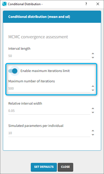
- Maximum number of iterations (default: 500, needs to be larger than the interval length, available if “enable maximum iterations limit’ is on): maximum number of iterations for the conditional distribution task. Even if the convergence criteria are not fulfilled, the algorithm stops after this maximum number of iterations. If the maximum number of iterations is reached, a warning message will be displayed in the interface.
 |
 |
|---|