Purpose
The figure displays the estimators of the individual parameters, and those for random effects, as a function of the covariates. It allows to identify correlation effects between the individual parameters and the covariates.
The estimators can be:
- simulated parameters: individual parameters and individual random effects are sampled from the distributions \(p(\psi_i|y_i;\hat{\theta})\) and \(p(\eta_i|y_i;\hat{\theta})\). These estimators lead to more reliable results, especially when individual data are sparse and the distributions of conditional modes and means of individual parameters are affected by shrinkage.
- the conditional means \(E(\psi_i|y_i;\hat{\theta})\) for parameters \(\psi_i\)and \(E(\eta_i|y_i;\hat{\theta})\) for random effects \(\eta_i\),
- the conditional modes of the same distributions.
On the boxplots for categorical covariates, red “+” are outlier points below Q1-1.5*IQR (interquartile range) or above Q3+1.5*IQR.
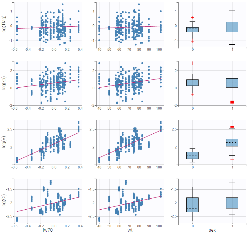
Identifying correlation effects
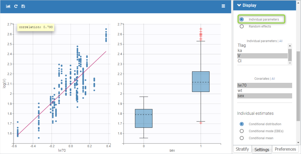
In the example below, we can see the parameters of a one-compartment PK model with delayed first-order absorption and linear elimination estimated on the warfarin data set. The simulated individual parmeters of the 4 parameters of the PK model are displayed with respect to the covariates: the weight wt, a transformed version of the weight (lw70=log(wt/70)) and the sex category.
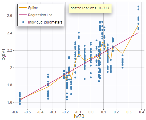
Visual guidelines
In order to help identifying correlations, regression lines, spline interpolations and Pearson correlation coefficients can be overlaid on the plots for continuous covariates. Here we can see a strong correlation between the parameter V and the covariate lw70.
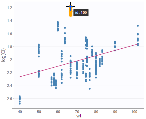
Highlight
Hovering on a point reveals the corresponding individual and, if multiple individual parameters have been simulated from the conditional distribution for each individual, highlights all the points points from the same individual. This is useful to identify possible outliers and subsequently check their behavior in the observed data.
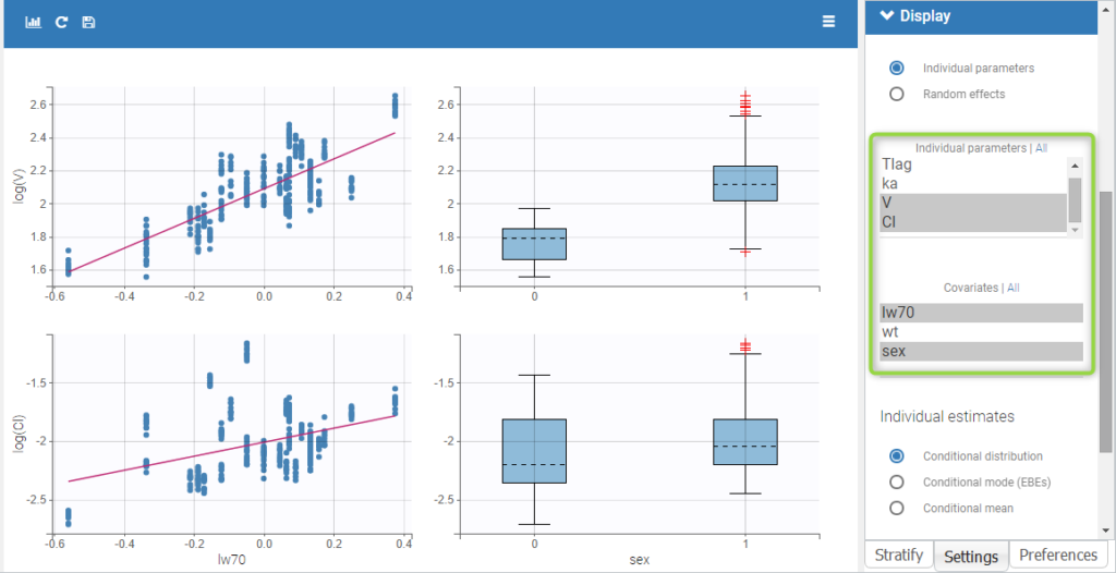
Selection
It is possible to select a subset of covariates or parameters, as shown below. In the selection panel, a set of contiguous rows can be selected with a single extended click, or a set of non-contiguous rows can be selected with several clicks while holding the Ctrl key. This is useful when there are many parameters or covariates. In particular, it is frequent to introduce transformed covariates, the selection allows to focus on the transformed versions rather than the original.
Comparing individual parameters and random effects
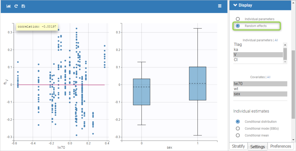
By default, the values on the Y-axis are computed with the individual parameters. One can choose to display the random effects instead. If some individual parameters are already modelled with covariates, this is taken into account by the random effects values, thus allowing to focus on remaining correlations.
The figures below show the diagnosis plots with individual parameters or random effects when the models for parameters V includes the covariate lw70. On the top, one can identify the correlations between individual parameters and covariates: the log-volume (log(V)) clearly increases with the log-transformed weight, as well with sex. On the other hand, the random effects on the bottom allow to focus on correlations that are not yet taken into account in the covariate model. Because the model already includes a linear relationship between the log-volume and the log-transformed weight, 
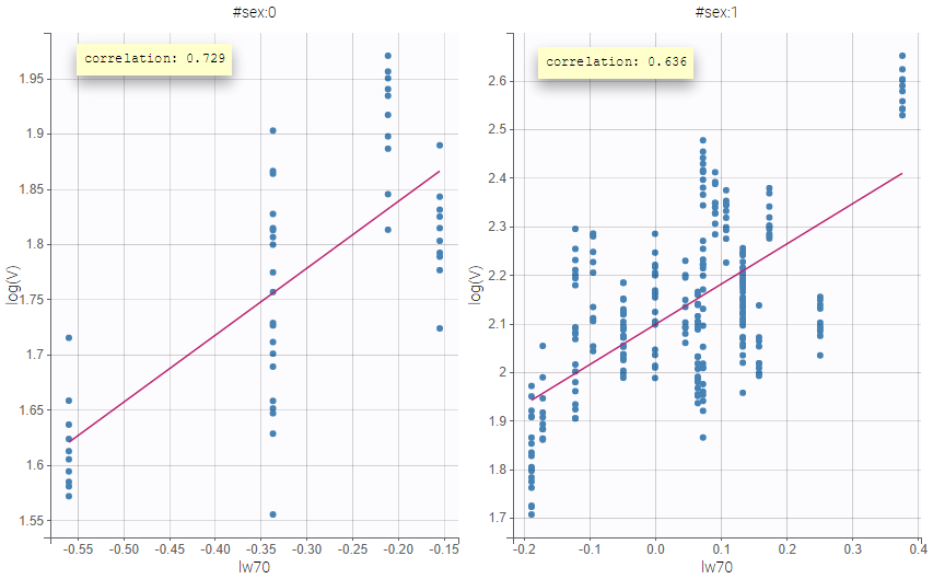
Stratification
Stratification can be applied by creating groups of covariate values. As can be seen below, these groups can then be split, colored or filtered, allowing to check the effect of the covariate on the correlation between two parameters. The correlation coefficient is updated according to the split or filtering.
Settings
- General
- Legend and grid : add/remove the legend or the grid. There is only one legend for all plots.
- Correlation: display/hide the correlation coefficient associated with each scatter plot.
- Display
- Y-axis. The user can choose to see either the individual parameters or the random effects.
- Selection. The user can select some of the parameters or covariates to display only the corresponding plots. A simple click selects one parameter (or covariate), whereas multiple clicks while holding the Ctrl key selects a set of parameters.
- Individual estimates. The user can define which estimators are used for the definition of the individual parameters and thus for the random effects (conditional mean, conditional mode, simulated parameters)
- Visual cues. Add/remove a regression line or a spline interpolation.
By default, all plots are proposed with simulated individual parameters.