1.Monolix Documentation
Version 2024
This documentation is for Monolix starting from 2018 version.
©Lixoft
Monolix
Monolix (Non-linear mixed-effects models or “MOdèles NOn LInéaires à effets miXtes” in French) is a platform of reference for model based drug development. It combines the most advanced algorithms with unique ease of use. Pharmacometricians of preclinical and clinical groups can rely on Monolix for population analysis and to model PK/PD and other complex biochemical and physiological processes. Monolix is an easy, fast and powerful tool for parameter estimation in non-linear mixed effect models, model diagnosis and assessment, and advanced graphical representation. Monolix is the result of a ten years research program in statistics and modeling, led by Inria (Institut National de la Recherche en Informatique et Automatique) on non-linear mixed effect models for advanced population analysis, PK/PD, pre-clinical and clinical trial modeling & simulation.
Objectives
The objectives of Monolix are to perform:
- Parameter estimation for nonlinear mixed effects models
- estimating the maximum likelihood estimator of the population parameters, without any approximation of the model (linearization, quadrature approximation, …), using the Stochastic Approximation Expectation Maximization (SAEM) algorithm,
- computing the conditional modes, sample from the conditional distribution to compute the conditional means and the conditional standard deviations of the individual parameters, using the Hastings-Metropolis algorithm
- estimating standard errors for the maximum likelihood estimator
- Model selection and diagnosis
- comparing several models using some information criteria (AIC, BIC)
- testing parameters using the Wald Test
- testing correlation using Pearson’s correlation test
- testing normality of distribution using Shapiro’s test.
- Easy description of pharmacometric models (PK, PK-PD, discrete data) with the Mlxtran language
- Goodness of fit plots
An interface for ease of use
Monolix can be used either via a graphical user interface (GUI) or a command-line interface (CLI) for powerful scripting. This means less programming and more focus on exploring models and pharmacology to deliver in time. The interface is depicted as follows: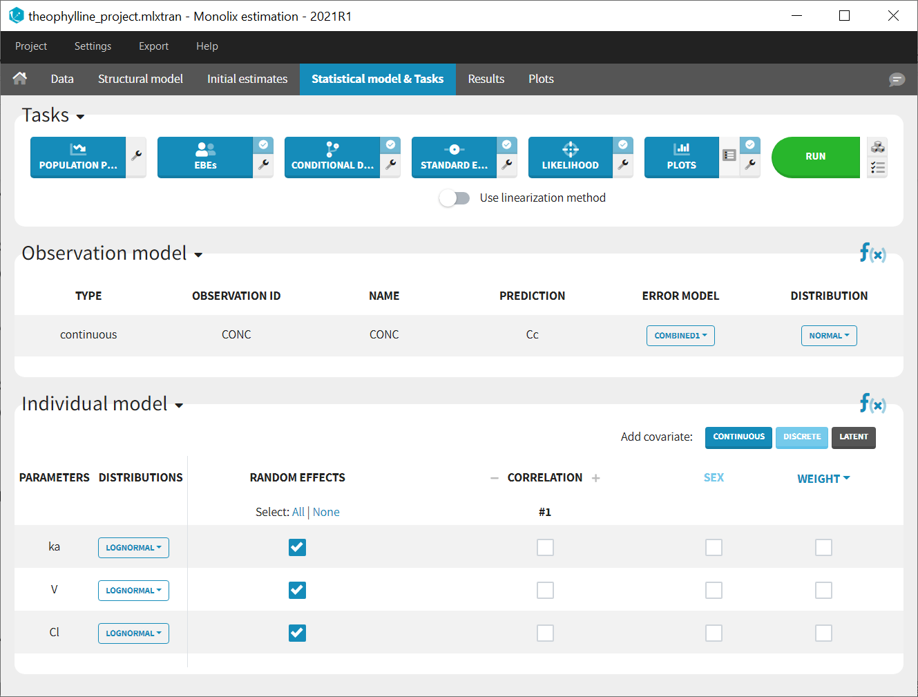
The GUI consists of 7 tabs.
- Welcome
- Data
- Structural model
- Initial estimates
- Tasks and statistical model
- Results
- Plots
Each of these tabs refer to a specific section on this website. An advanced description of available plots is also provided.
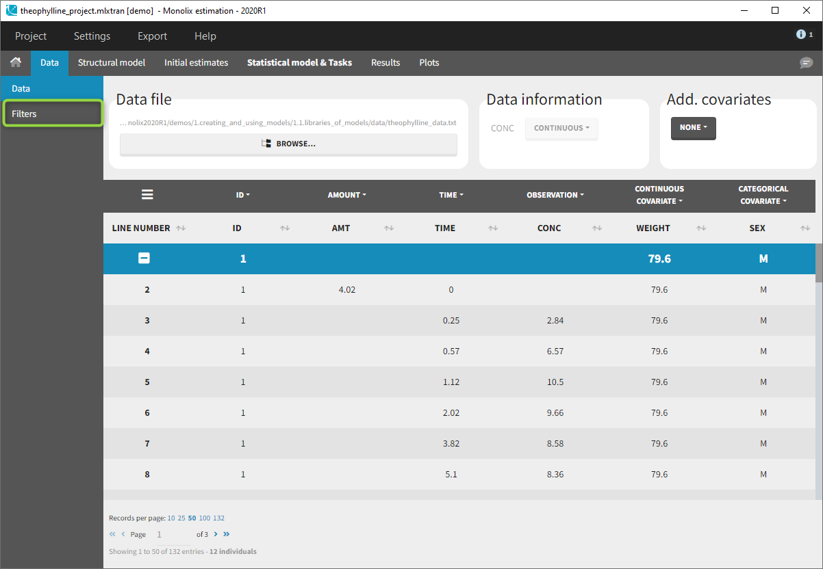
2.Data
2.1.Defining a data set
To start a new Monolix project, you need to define a dataset by loading a file in the Data tab, and load a model in the structural model tab. The project can be saved only after defining the data and the model.
Supported file types: Supported file types include .txt, .csv, and .tsv files. Starting with version 2024, additional Excel and SAS file types are supported: .xls, .xlsx, .sas2bdat, and .xpt files in addition to .txt, .csv, and .tsv files.
The data set format expected in the Data tab is the same as for the entire MonolixSuite, to allow smooth transitions between applications. The columns available in this format and example datasets are detailed on this page. Briefly:
- Each line corresponds to one individual and one time point
- Each line can include a single measurement (also called observation), or a dose amount (or both a measurement and a dose amount)
- Dosing information should be indicated for each individual, even if it is identical for all.
Your dataset may not be originally in this format, and you may want to add information on dose amounts, limits of quantification, units, or filter part of the dataset. To do so, you should proceed in this order:
- Formatting: If needed, format your data first by loading the dataset in the Data Formatting tab. Briefly, it allows to:
- to deal with several header lines
- merge several observation columns into one
- add censoring information based on tags in the observation column
- add treatment information manually or from external sources
- add more columns based on another file
- Loading a new data set: If the data is already in the right format, load it directly in the Data tab (otherwise use the formatted dataset created by data formatting).
- Observation types: Specify if the observation is of type continuous, count/categorical or event.
- Labeling: label the columns not recognized automatically to indicate their type and click on ACCEPT.
- Filtering: If needed, filter your dataset to use only part of it in the Filters tab
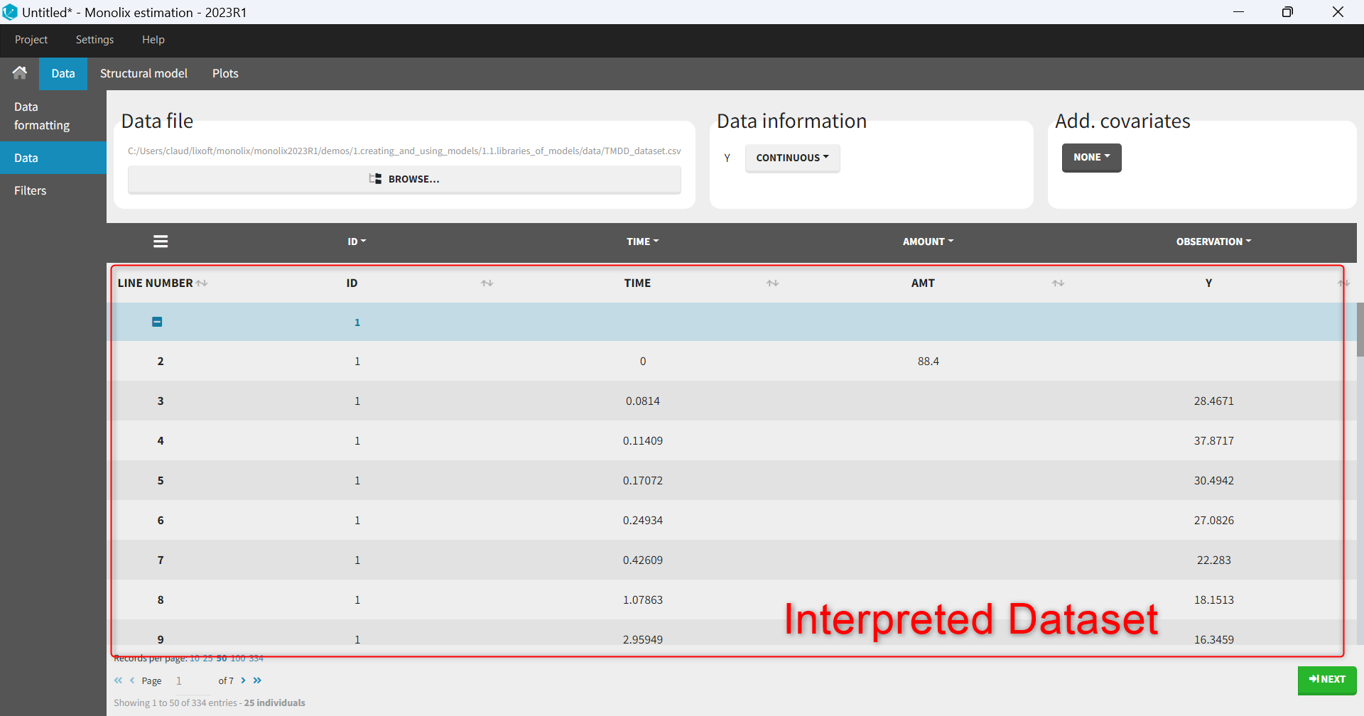
- Explore: The interpreted dataset is displayed in Data, and Plots and covariate statistics are generated.
If you have already defined a dataset in Datxplore or in PKanalix, you can skip all those steps in Monolix and create a new project by importing a project from Datxplore or PKanalix.
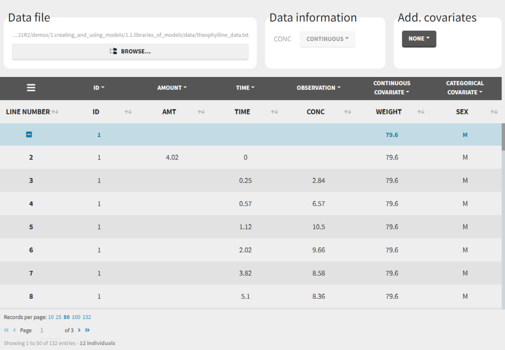
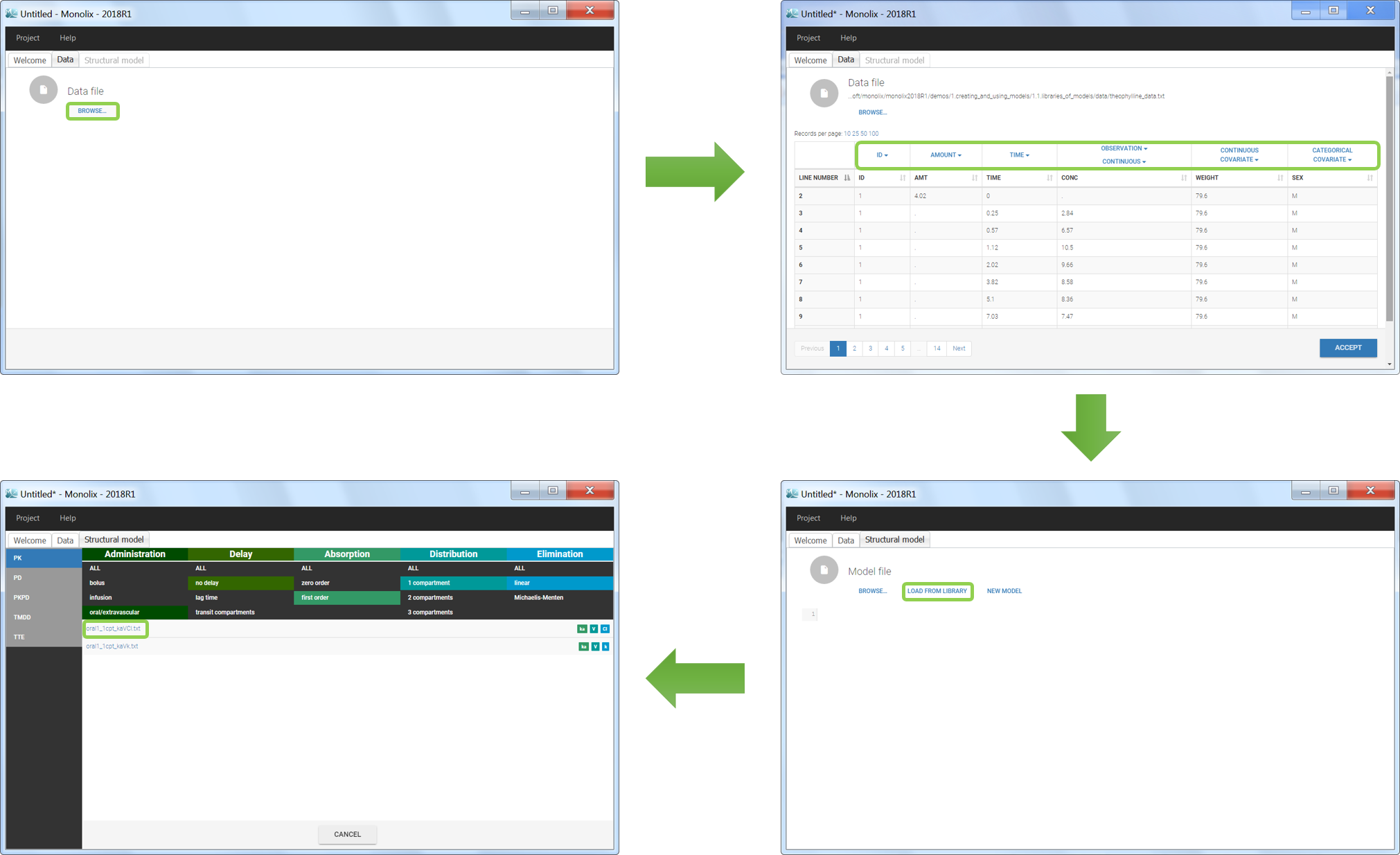
Loading a new data set
To load a new data set, you have to go to “Browse” your data set (green frame), tag all the columns (purple frame), define the observation types in Data Information (blue frame), and click on the blue button ACCEPT as on the following. If the dataset does not follow a formatting rule, the dataset will not be accepted, but errors will guide you to find what is missing and could be added by data formatting.
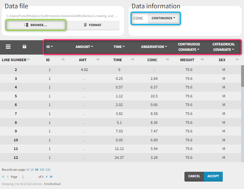
Observation types
There are three types of observations:
- continuous: The observation is continuous and can take any value within a range. For example, a concentration is a continuous observation.
- count/categorical: The observation values can take values only in a finite categorical space. For example, the observation can be a categorical observation (an effect can be observed as “low”, “medium”, or “high”) or a count observation over a defined time (the number of epileptic crisis in a week).
- event: The observation is an event, for example the time of death.
For each OBSERVATION ID, the type of observations must be specified by the user in the interface. Depending on the choice, the data will be displayed in the Observed Data plot in different ways (e.g spaghetti plot for continuous data and Kaplan-Meier plot for event data). The mapping of model outputs and observations from the dataset will also take into account the data type (e.g a model outptu of type “event” can only be mapped to an observation that is also an “event”). Once a model has been selected, the choice of the data types are locked (because they are enforced by the model output type).
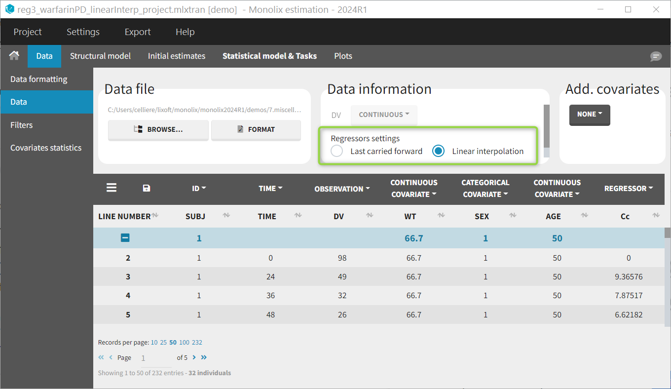
Regressor settings
If columns have been tagged as REGRESSORS, the interpolation method for the regressors can be chosen. In the dataset, regressors are defined only for a finite number of time points. In between those time points, the regressor values can be interpolated in two different ways:
- last carried forward: if we have defined in the dataset two times for each individual with \(reg_A\) at time \(t_A\) and \(reg_B\) at time \(t_B\)
- for \(t\le t_A\), \(reg(t)=reg_A\) [first defined value is used]
- for \(t_A\le t<t_B\), \(reg(t)=reg_A\) [previous value is used]
- for \(t>t_B\), \(reg(t)=reg_B\) [previous value is used]
- linear interpolation: the interpolation is:
- for \(t\le t_A\), \(reg(t)=reg_A\) [first defined value is used]
- for \(t_A\le t<t_B\), \(reg(t)=reg_A+(t-t_A)\frac{(reg_B-reg_A)}{(t_B-t_A)}\) [linear interpolation is used]
- for \(t>t_B\), \(reg(t)=reg_B\) [previous value is used]
The interpolation is used to obtain the regressor value at times not defined in the dataset. This is necessary to integrate ODE-based models (which are using an internal adaptative time step), or obtain prediction on a fine grid for the plots (e.g in the Individuals fits) for instance.
When some dataset lines have a missing regressor value (dot “.”), the same interpolation method is used.
Labeling (column tagging)
The column type suggested automatically by Monolix based on the headers in the data can be customized in the preferences. By clicking on Settings>Preferences, the following windows pops up.
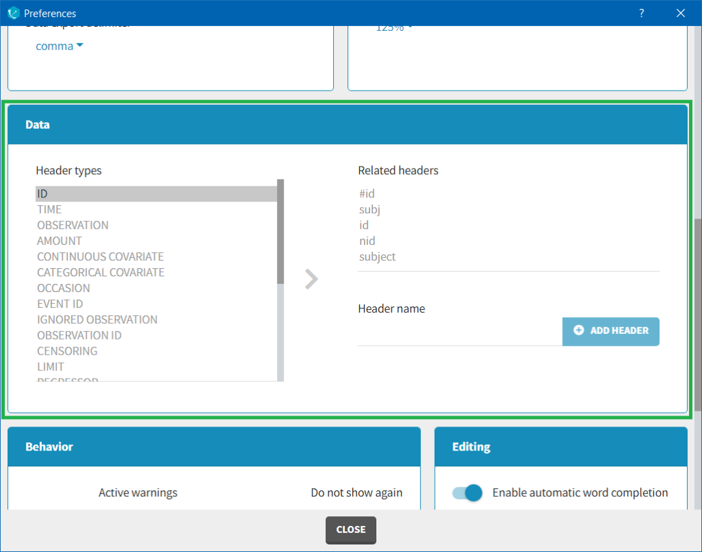
In the DATA frame, you can add or remove preferences for each column.
To remove a preference, double-click on the preference you would like to remove. A confirmation window will be proposed.
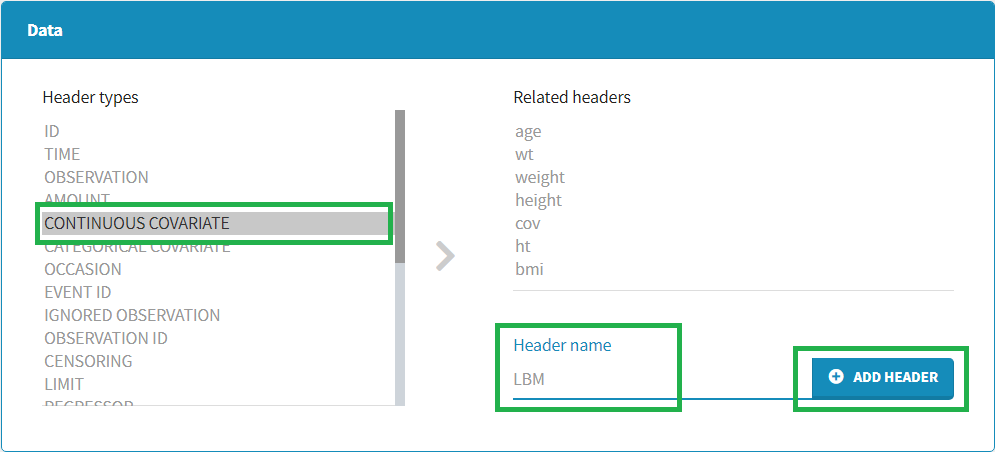
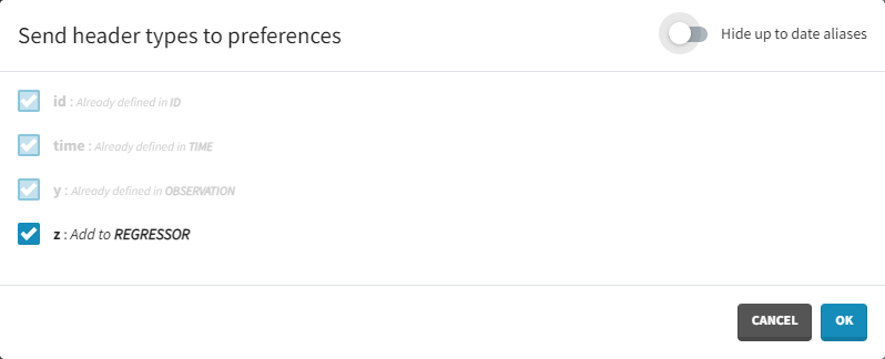
To add a preference, click on the header type you consider, add a name in the header name and click on “ADD HEADER” as on the following figure.
Notice that all the preferences are shared between Monolix, Datxplore, and PKanalix.
Starting from the version 2024, it is also possible to update the preferences with the columns tagged in the opened project, by clicking on the icon in the top left corner of the table:
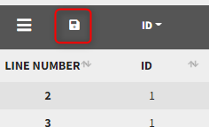
Clicking on the icon will open a modal with the option to choose which of the tagged headers a user wants to add to preferences:
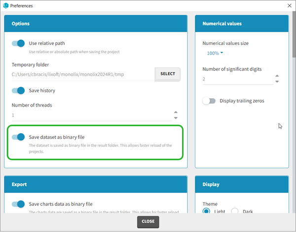
Dataset load times
Starting with the 2024 version, it is possible to improve the project load times, especially for projects with large datasets, but saving the data as a binary file. This option is available in Settings>Preferences and will save a copy of the data file in binary format in the results folder. When reloading a project, the dataset will be read from the binary file, which will be faster. If the original dataset file has been modified (compared to the binary), a warning message will appear, the binary dataset will not be used and the original dataset fiel will be loaded instead.
Resulting plots and tables to explore the data
Once the dataset is accepted:
- Plots are automatically generated based on the interpreted dataset to help you proceed with a first data exploration before running any task.
- The interpreted dataset appears in Data tab, which incorporates all changes after formatting and filtering.
- Covariate Statistics appear in a section of the data tab.
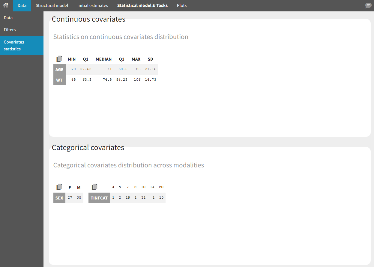
All the covariates (if any) are displayed and a summary of the statistics is proposed. For continuous covariates, minimum, median and maximum values are proposed along with the first and third quartile, and the standard deviation. For categorical covariates, all the modalities are displayed along with the number of each. Note the “Copy table” button that allows to copy the table in Word and Excel. The format and the display of the table will be preserved.
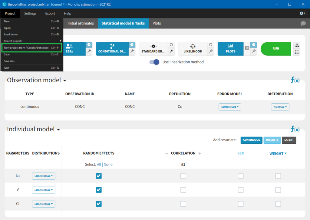
Importing a project from Datxplore or PKanalix
It is possible to import a project from Datxplore or PKanalix. For that, go to Project>New project for Datxplore/PKanalix (as in the green box of the following figure). In that case, a new project will be created and all the DATA frame will already be filled by the information from the Datxplore or PKanalix project.
2.2.Data Format
- Each line corresponds to one individual and one time point.
- Each line can include a single measurement (also called observation), or a dose amount (or both a measurement and a dose amount).
- Dosing information should be indicated for each individual in a specific column, even if it is the same treatment for all individuals.
- Headers are free but there can be only one header line.
- Different types of information (dose, observation, covariate, etc) are recorded in different columns, which must be tagged with a column type (see below).
 Notice that Monolix often provides an initial guess of the type of the column depending on the name.
Description of column-types
The first line of the data set must be a header line, defining the names of the columns. The columns names are completely free. In the MonolixSuite applications, when defining the data, the user will be asked to assign each column to a column-type (see here for an example of this step). The column type will indicate to the application how to interpret the information in that column. The available column types are given below. Column-types used for all types of lines:- ID (mandatory): identifier of the individual
- OCCASION (formerly OCC): identifier (index) of the occasion
- TIME: time of the dose or observation record
- DATE/DAT1/DAT2/DAT3: date of the dose or observation record, to be used in combination with the TIME column
- EVENT ID (formerly EVID): identifier to indicate if the line is a dose-line or a response-line
- IGNORED OBSERVATION (formerly MDV): identifier to ignore the OBSERVATION information of that line
- IGNORED LINE (from 2019 version): identifier to ignore all the information of that line
- CONTINUOUS COVARIATE (formerly COV): continuous covariates (which can take values on a continuous scale)
- CATEGORICAL COVARIATE (formerly CAT): categorical covariate (which can only take a finite number of values)
- REGRESSOR (formerly X): defines a regression variable, i.e a variable that can be used in the structural model (used e.g for time-varying covariates)
- IGNORE: ignores the information of that column for all lines
- OBSERVATION (mandatory, formerly Y): records the measurement/observation for continuous, count, categorical or time-to-event data
- OBSERVATION ID (formerly YTYPE): identifier for the observation type (to distinguish different types of observations, e.g PK and PD)
- CENSORING (formerly CENS): marks censored data, below the lower limit or above the upper limit of quantification
- LIMIT: upper or lower boundary for the censoring interval in case of CENSORING column
- AMOUNT (formerly AMT): dose amount
- ADMINISTRATION ID (formerly ADM): identifier for the type of dose (given via different routes for instance)
- INFUSION RATE (formerly RATE): rate of the dose administration (used in particular for infusions)
- INFUSION DURATION (formerly TINF): duration of the dose administration (used in particular for infusions)
- ADDITIONAL DOSES (formerly ADDL): number of doses to add in addition to the defined dose, at intervals INTERDOSE INTERVAL
- INTERDOSE INTERVAL (formerly II): interdose interval for doses added using ADDITIONAL DOSES or STEADY-STATE column types
- STEADY STATE (formerly SS): marks that steady-state has been achieved, and will add a predefined number of doses before the actual dose, at interval INTERDOSE INTERVAL, in order to achieve steady-state
Order of events
There are prioritization rules in place in case of various event types occurring at the same time. The order of row numbers in the data set is not important, and same is true for the order of administration and empty/reset macros in model files. The sequence of events will always be the following:- regressors are updated,
- reset done by EVID=3 or EVID=4 is performed,
- dose is administered,
- empty/reset done by macros is performed,
- observation is made.
2.3.Data formatting
The dataset format that is used in Monolix is the same as for the entire MonolixSuite, to allow smooth transitions between applications. In this format, some rules have to be fullfilled, for example:
- Each line corresponds to one individual and one time point.
- Each line can include a single measurement (also called observation), or a dose amount (or both a measurement and a dose amount).
- Dose amount should be indicated for each individual dose in a column AMOUNT, even if it is identical for all.
- Headers are free but there can be only one header line.
If your dataset is not in this format, in most cases, it is possible to format it in a few steps in the data formatting tab, to incorporate the missing information.
In this case, the original dataset should be loaded in the “Format data” box, or directly in the “Data Formatting” tab, instead of the “Data” tab. In the data formatting module, you will be guided to build a dataset in the MonolixSuite format, starting from the loaded csv file. The resulting formatted dataset is then loaded in the Data tab as if you loaded an already-formatted dataset in “Data” directly. Then as for defining any dataset, you can tag columns, accept the dataset, and once accepted, the Filters tab can be used to select only parts of this dataset for analysis. Note that units and filters are neither information to be included in the data file, nor part of the data formatting process.
Jump to:
- Data formatting workflow
- Dataset initialization (mandatory step)
- Selecting header lines or lines to exclude to merge header lines or exclude a line
- Tagging mandatory columns such as ID and TIME
- Initialization example
- Creating occasions from a SORT column to distinguish different sets of measurements within each subject, (eg formulations).
- Selecting an observation type (required to add a treatment)
- Merging observations from several columns
- As observation ids to map them to several outputs of a joint model
- As occasions
- Option “Duplicate information from undefined columns”
- As observation ids to map them to several outputs of a joint model
- Specifying censoring from censoring tags eg “BLQ” instead of a number in an observation column. Demo project DoseAndLOQ_manual.mlxtran
- Adding doses in the dataset Demo project DoseAndLOQ_manual.mlxtran
- Reading censoring limits or dosing information from the dataset “by category” or “from data”. Demo projects DoseAndLOQ_byCategory.mlxtran and DoseAndLOQ_fromData.mlxtran
- Creating occasions from dosing intervals to analyze separately the measurements following different doses.Demo project doseIntervals_as_Occ.mlxtran
- Handling urine data to merge start and end times in a single column.
- Adding new columns from an external file, eg new covariates, or individual parameters estimated in a previous analysis. Demo warfarin_PKPDseq_project.mlxtran
- Exporting the formatted dataset
1. Data formatting workflow
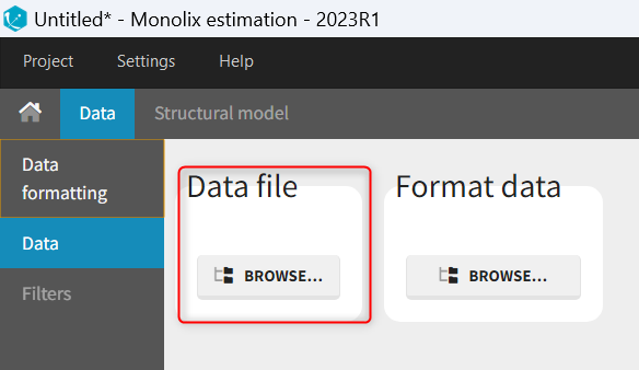
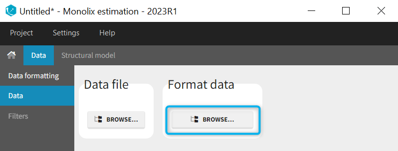 When opening a new project, two Browse buttons appear. The first one, under “Data file”, can be used to load a dataset already in a MonolixSuite-standard format, while the second one, under “Format data”, allows to load a dataset to format in the Data formatting module.
After loading a dataset to format, data formatting operations can be specified in several subtabs: Initialization, Observations, Treatments and Additional columns.
- Initialization is mandatory and must be filled before using the other subtabs.
- Observations is required to enable the Treatments tab.
After Initialization has been validated by clicking on “Next”, a button “Preview” is available from any subtab to view in the Data tab the formatted dataset based on the formatting operations currently specified.


2. Dataset initialization
The first tab in Data formatting is named Initialization. This is where the user can select header lines or lines to exclude (in the blue area on the screenshot below) or tag columns (in the yellow area).
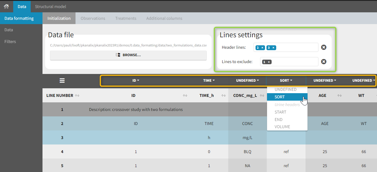
Selecting header lines or lines to exclude
These settings should contain line numbers for lines that should be either handled as column headers or that should be excluded.
- Header lines: one or several lines containing column header information. By default, the first line of the dataset is selected as header. If several lines are selected, they are merged by data formatting into a single line, concatenating the cells in each column.
- Lines to exclude (optional): lines that should be excluded from the formatted dataset by data formatting.
Tagging mandatory columns
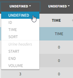
Only the columns corresponding to the following tabs must be tagged in Initialization, while all the other columns should keep the default UNDEFINED tag:
- ID (mandatory): subject identifiers
- TIME (mandatory): the single time column
- SORT (optional): one or several columns containing SORT variables can be tagged as SORT. Occasions based on these columns will be created in the formatted dataset as described in Section 3.
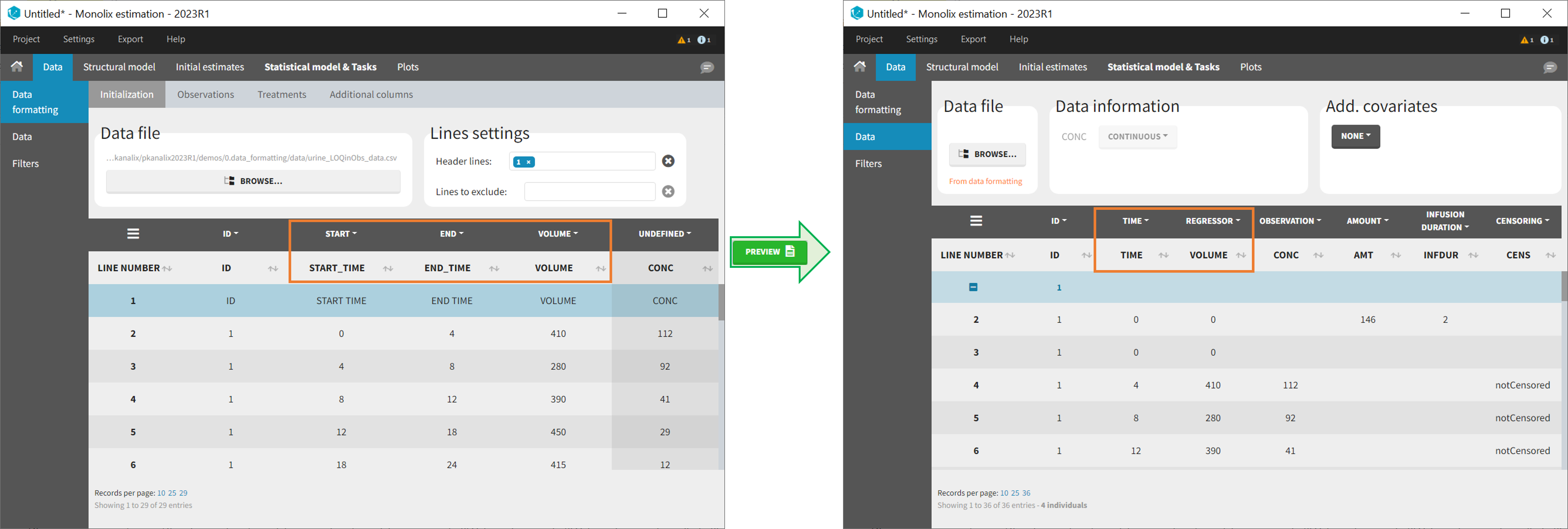
- START, END and VOLUME (mandatory in case of urine data): these column tags replace the TIME tag in case of urine data, if the urine collection time intervals are encoded in the dataset with two time columns for the start and end times of the intervals. In that case there should also be a column with the urine volume in each interval. See Section 10 for more details.
Initialization example
- demo CreateOcc_AdmIdbyCategory.pkx (Monolix demo in the folder 0.data_formatting, here imported into Monolix. The screenshot below focuses on the formatting initialization and excludes other elements present in the demo):
In this demo the first line of the dataset is excluded because it contains a description of the study. The second line contains column headers while the third line contains column units. Since the MonolixSuite-standard format allows only a single header line, lines 2 and 3 are merged together in the formatted dataset.
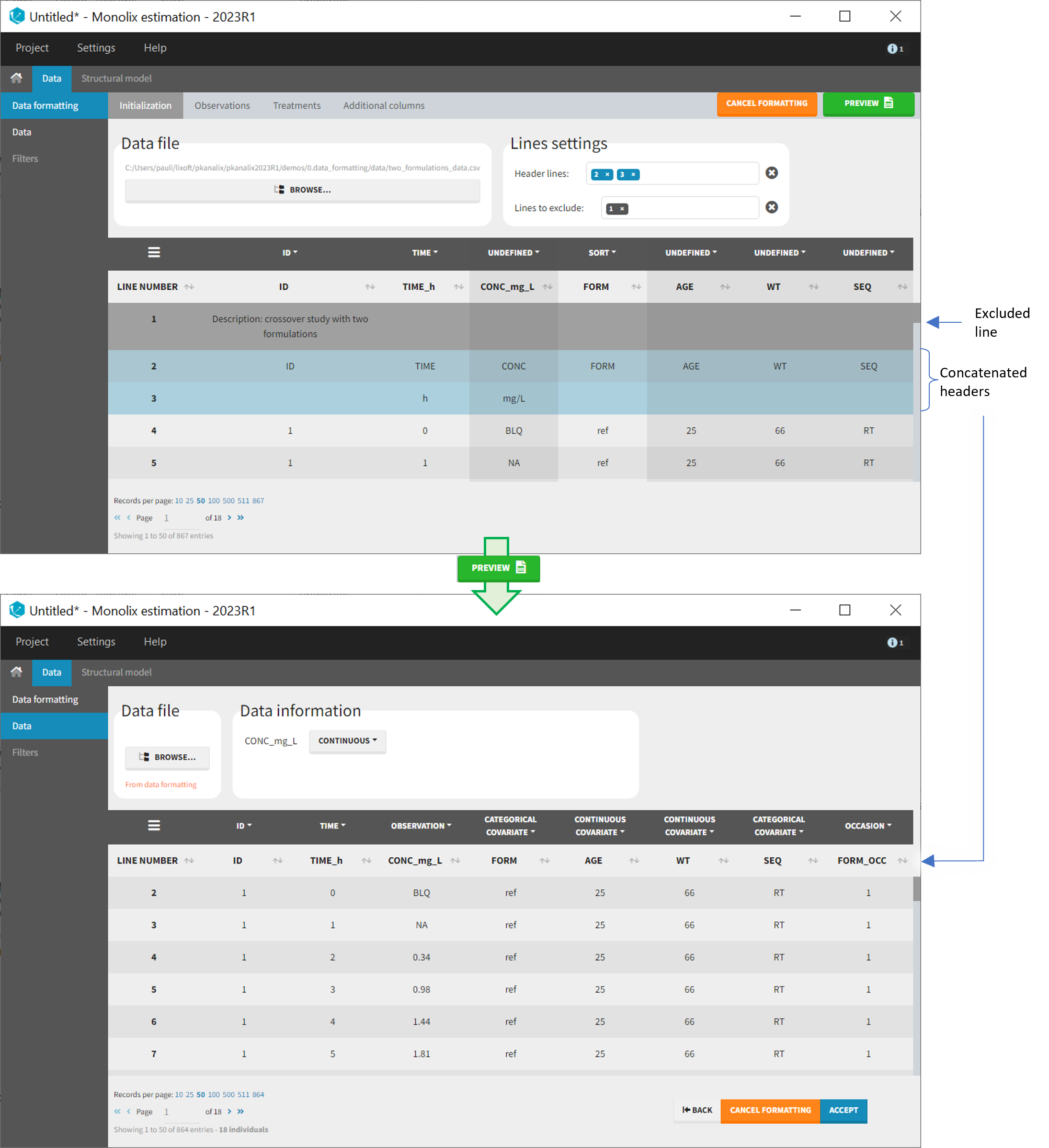
3. Creating occasions from a SORT column
A SORT variable can be used to distinguish different sets of measurements (usually concentrations) within each subject, that should be analyzed separately by Monolix (for example: different formulations given to each individual at different periods of time, or multiple doses where concentration profiles are available to be analyzed following several doses).
In Monolix, these different sets of measurements must be distinguished as OCCASIONS (or periods of time), via the OCCASION column-type. However, a column tagged as OCCASION can only contain integers with occasion indexes. Thus, if a column with a SORT variable contains strings, its format must be adapted by Data formatting, in the following way:

- the user must tag the column as SORT in the Initialization subtab of Data formatting,
- the user validates the Initialization with “Next”, then clicks on “Preview” (after optionally defining other data formatting operations),
- the formatted data is shown in Data: the column tagged as SORT is automatically duplicated. The original column is automatically tagged as CATEGORICAL COVARIATE in Data, while the duplicated column, which has the same name appended with “_OCC”, is tagged as OCCASION. This column contains occasion indexes instead of strings.
Example:
- demo CreateOcc_AdmIdbyCategory.pkx (PKanalix demo in the folder 0.data_formatting, here imported into Monolix. The screenshot below focuses on the formatting of occasions and excludes other elements present in the demo):
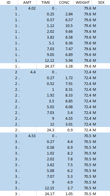
The image below shows lines 25 to 29 from the dataset from the CreateOcc_AdmIdbyCategory.pkx demo, where covariate columns have been removed to simplify the example. This dataset contains two sets of concentration measurements for each individual, corresponding to two different drug formulations administered on different periods. The sets of concentrations are distinguished with the FORM column, which contains “ref” and “test” categories (reference/test formulations). The column is tagged as SORT in Data formatting Initialization. After clicking on “Preview”, we can see in the Data tab that a new column named FORM_OCC has been created with occasion indexes for each individual: for subject 1, FORM_OCC=1 corresponds to the reference formulation because it appears first in the dataset, and FORM_OCC=2 corresponds to the test formulation because it appears in second in the dataset.

4. Selecting an observation type
The second subtab in Data formatting allows to select one or several observation types. An observation type corresponds to a column of the dataset, that contains a type of measurements (usually drug concentrations, but it can also be PD measurements for example). Only columns that have not been tagged as ID, TIME or SORT are available as observation type. 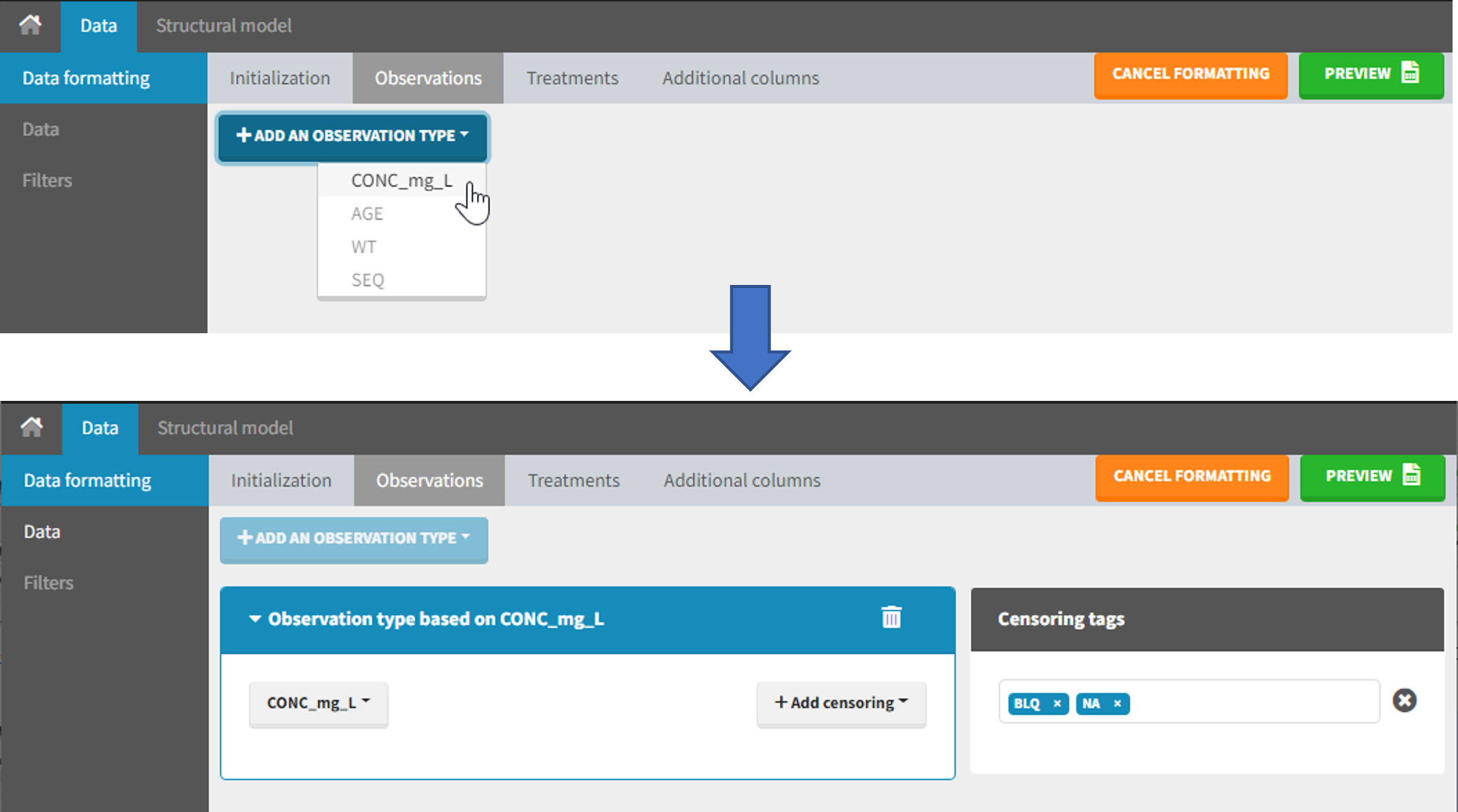
This action is optional and can have several purposes:
- If doses must be added by Data formatting (see Section 7), specifying the column containing observations is mandatory, to avoid duplicating observations on new dose lines.
- If several observation types exist in different columns (for example: concentrations for different analytes, or measurements for PK and PD), they must be specified in Data formatting to be merged into a single observation column (see Section 5).
- In the MonolixSuite-standard format, the column containing observations can only contain numbers, and no string except “.” for a missing observation. Thus if this column contains strings in the original dataset, it must be adapted by Data formatting, with two different cases:
- if the strings are tags for censored observations (usually BLQ: below the limit of quantification), they can be specified in Data formatting to adapt the encoding of the censored observations (see Section 6),
- any other string in the column is automatically replaced by “.” by Data formatting.
5. Merging observations from several columns
The MonolixSuite-standard format allows a single column containing all observations (such as concentrations or PD measurements). Thus if a dataset contains several observation types in different columns (for example: concentrations for different analytes, or measurements for PK and PD), they must be specified in Data formatting to be merged into a single observation column.
In that case, different settings can be chosen in the area marked in orange in the screenshot below:
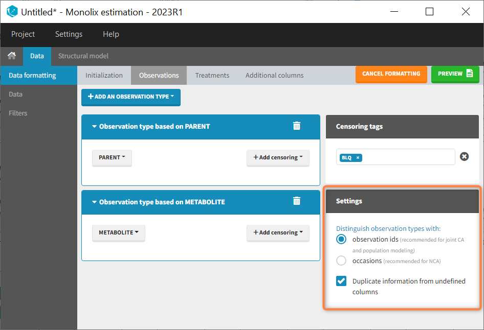
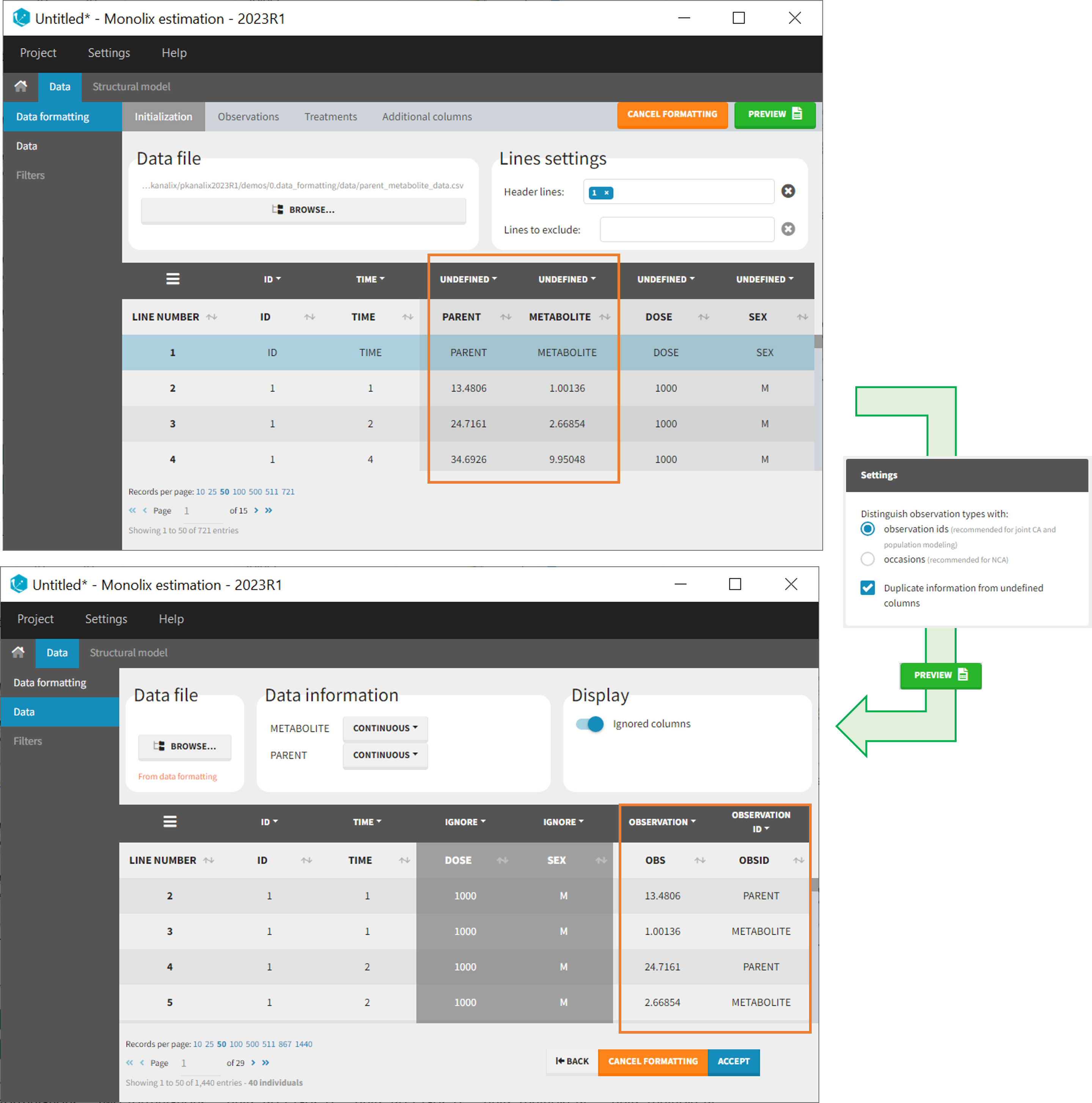
- The user must choose between distinguishing observation types with observation ids or occasions.
- The user can unselect the option “Duplicate information from undefined columns”.
As observation ids
After selecting the “Distinguish observation types with: observation ids” option and clicking “Preview,” the columns for different observation types are combined into a single column called “OBS.” Each row of the dataset is duplicated for each observation type, with one value per observation type. Additionally, an “OBSID” column is created, with the name of the observation type corresponding to the measurement on each row.
This option is recommended for joint modeling of observation types, such as CA in Monolix or population modeling in Monolix. It is important to note that NCA cannot be performed on two different observation ids simultaneously, so it is necessary to choose one observation id for the analysis.
Example:
- demo merge_obsID_ParentMetabolite.pkx PKanalix demo in the folder 0.data_formatting, here imported into Monolix. The screenshot below focuses on the formatting of observations and excludes other elements present in the demo):
This demo involves two columns that contain drug parent and metabolite concentrations. When merging both observation types with observation ids, a new column called OBSID is generated with categories labeled as “PARENT” and “METABOLITE.”
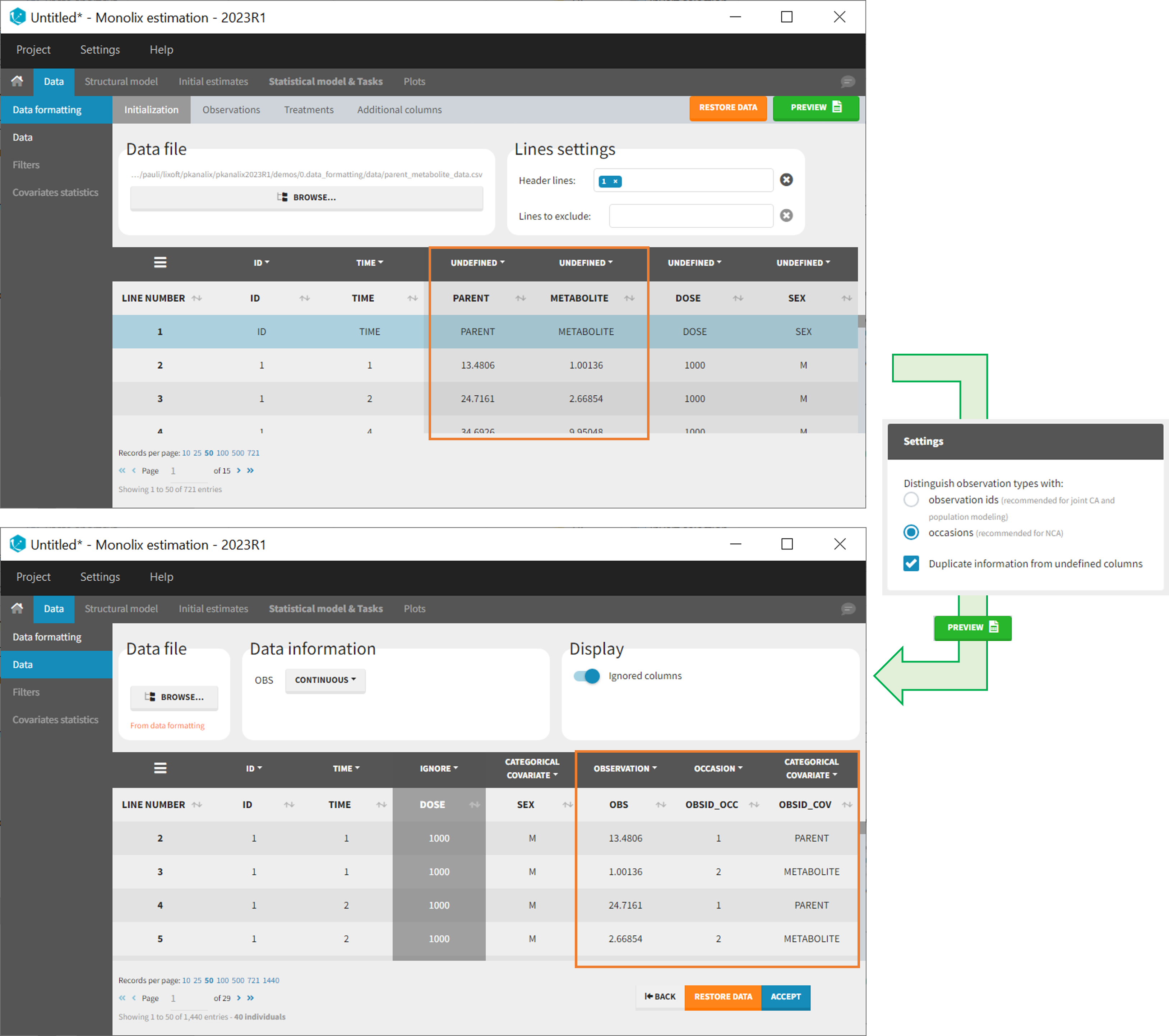
As occasions
After selecting the “Distinguish observation types with: occasions” option and clicking “Preview,” the columns for different observation types are combined into a single column called “OBS.” Each row of the dataset is duplicated for each observation type, with one value per observation type. Additionally, two columns are created: an “OBSID_OCC” column with the index of the observation type corresponding to the measurement on each row, and an “OBSID_COV” with the name of the observation type.
This option is recommended for NCA, which can be run on different occasions for each individual. However, joint modeling of the observation types with CA or population modeling with Monolix cannot be performed with this option.
Example:
- demo merge_occ_ParentMetabolite.pkx (PKanalix demo in the folder 0.data_formatting, here imported into Monolix. The screenshot below focuses on the formatting of observations and excludes other elements present in the demo):
This demo involves two columns that contain drug parent and metabolite concentrations. When merging both observation types with occasions, two new columns called OBSID_OCC and OBSID_COV are generated with OBSID_OCC=1 corresponding to OBSID_COV=”PARENT” catand OBSID_OCC=2 corresponding to OBSID_COV=”METABOLITE.”
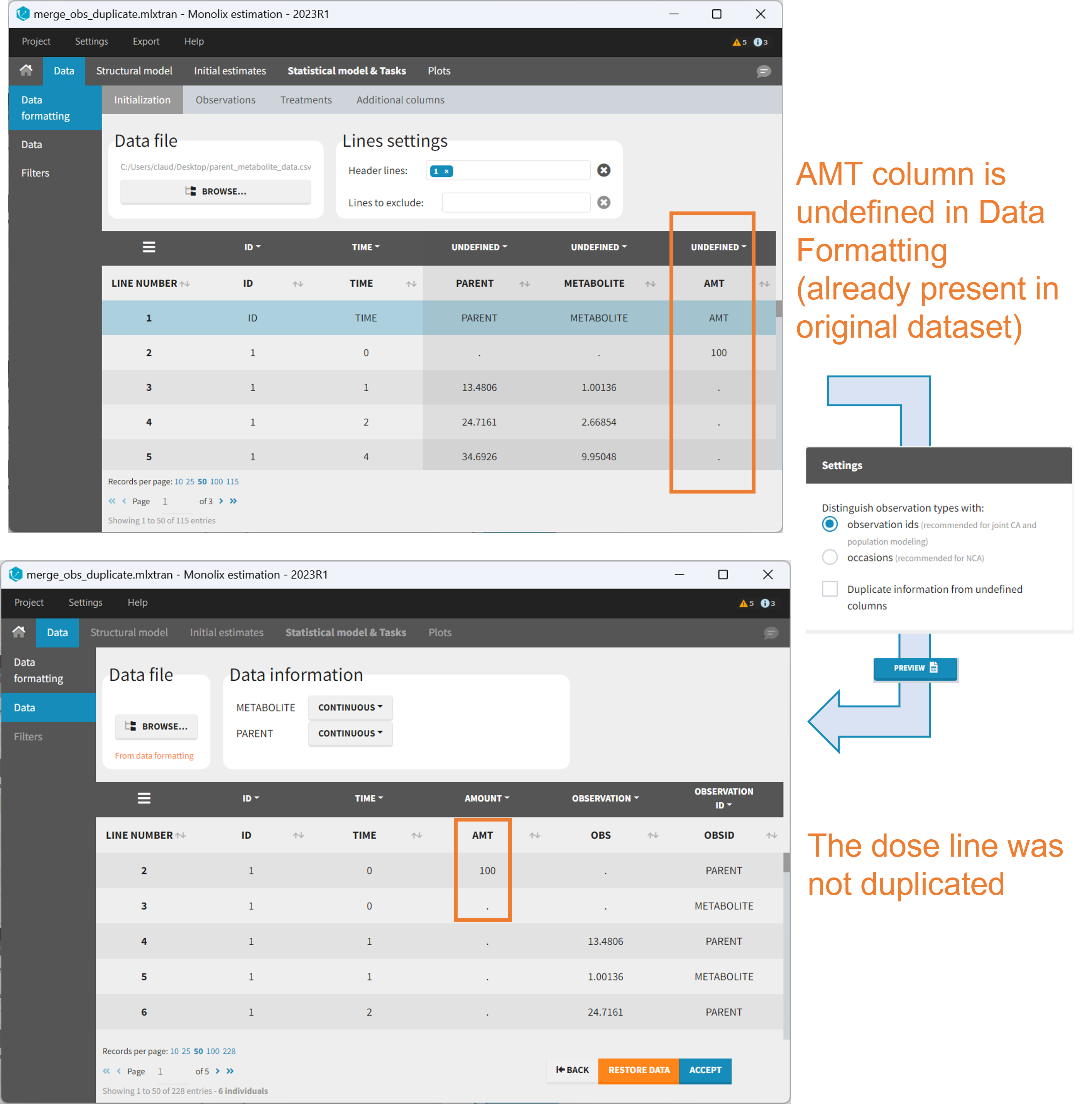
Duplicate information from undefined columns
When merging two observation columns into a single column, all other columns will see their lines duplicated. The data formatting will know how to treat columns which have been tagged in the Initialization tab, but not the other columns (header “UNDEFINED”) which are not used for data formatting. A checkbox enables to decide if the information from these columns should be duplicated on the new lines, or if “.” should be used instead. The default option is to duplicate information, because in general, the undefined columns correspond to covariates with one value per individual, so this value is the same for the two lines that correspond to the same id.

It is rare that you need to uncheck this box. An example where you should not duplicate the information is if you already have a column Amount in the MonolixSuite format, so with a dose amount only at the dosing time, and “.” everywhere else. If you do not want to specify amount again in data formatting, and simply want to merge observation columns as observation ids, you should not duplicate the lines of the Amount column which is undefined. Indeed, the dose amounts have been administered only once.
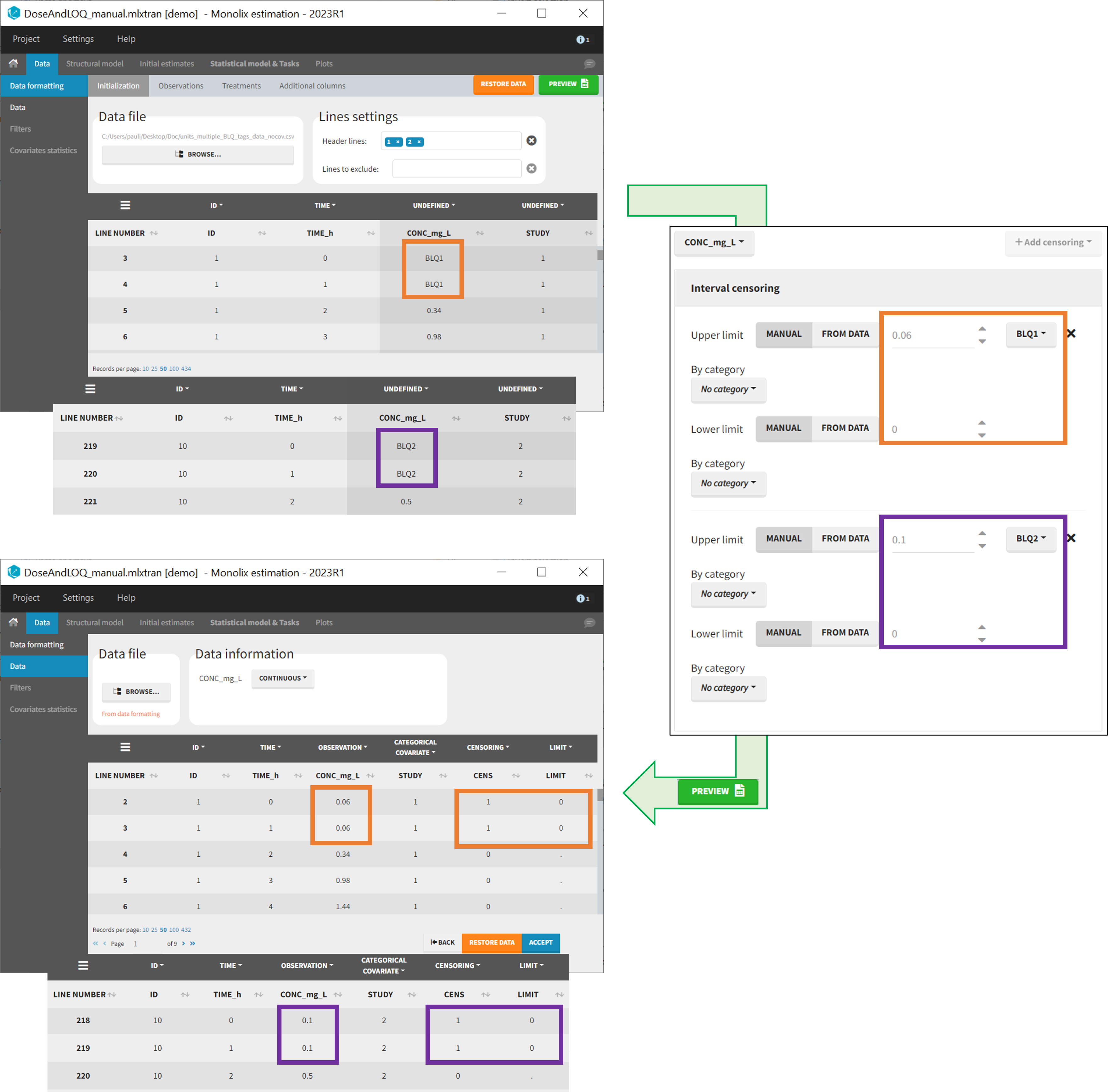
6. Specifying censoring from censoring tags
In the MonolixSuite-standard format, censored observations are encoded with a 1or -1 flag in a column tagged as CENSORING in the Data tab, while exact observations have a 0 flag in that column. In addition, on rows for censored observations, the LOQ is indicated in the observation column: it is the LLOQ (lower limit of quantification) if CENSORING=1 or the ULOQ (upper limit of quantification) if CENSORING=-1. Finally, to specify a censoring interval, an additional column tagged as LIMIT in the Data tab must exist in the dataset, with the other censoring bound.
The Data Formatting module can take as input a dataset with censoring tags directly in the observation column, and adapt the dataset format as described above. After selecting one or several observation types in the Observations subtab (see Section 4), all strings found in the corresponding columns are displayed in the “Censoring tags” on the right of the observation types. If at least one string is found, the user can then define some censoring associated with an observation type and with one or several censoring tags with the button “Add censoring”. 3 types of censoring can be defined:
- LLOQ: this corresponds to left-censoring, where the censored observation is below a lower limit of quantification (LLOQ), that must specified by the user. In that case Data Formatting replaces the censoring tags in the observation column by the LLOQ, and creates a new CENS column tagged as CENSORING in the Data tab, with 1 on rows that had censoring tags before formatting, and 0 on other rows.
- ULOQ: this corresponds to right-censoring, where the censored observation is above an upper limit of quantification (ULOQ), that must specified by the user. Here Data Formatting replaces the censoring tags in the observation column by the ULOQ, and creates a new CENS column tagged as CENSORING in the Data tab, with -1 on rows that had censoring tags before formatting, and 0 on other rows.
- Interval: this is for interval-censoring, where the user must specify two bound of a censoring interval, to which the censored observation belong. Data Formatting replaces the censoring tags in the observation column by the upper bound of the interval, and creates two new columns: a CENS column tagged as CENSORING in the Data tab, with 1 on rows that had censoring tags before formatting, and 0 on other rows, and a LIMIT column with the lower bound of the censoring interval on rows that had censoring tags before formatting, and “.” on other rows.
For each type of censoring, available options to define the limits are:
- “Manual“: limits are defined manually, by entering the limit values for all censored observations.
- “By category“: limits are defined manually for different categories read from the dataset.
- “From data“: limits are directly read from the dataset.
The options “by category” and “from data” are described in detail in Section 8.
Example:
- demo DoseAndLOQ_manual.mlxtran (the screenshot below focuses on the formatting of censored observations and excludes other elements present in the demo):
In this demo there are two censoring tags in the CONC column: BLQ1 (from Study 1) and BLQ2 (from Study 2), that correspond to different LLOQs. An interval censoring is defined for each censoring tag, with manual limits, where LLOQ=0.06 for BLQ1 and LLOQ=0.1 for BLQ2, and the lower limit of the censoring interval being 0 in both cases.
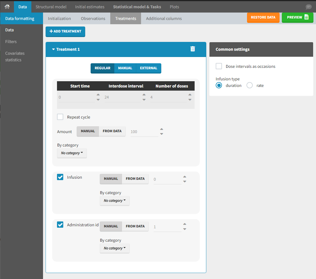
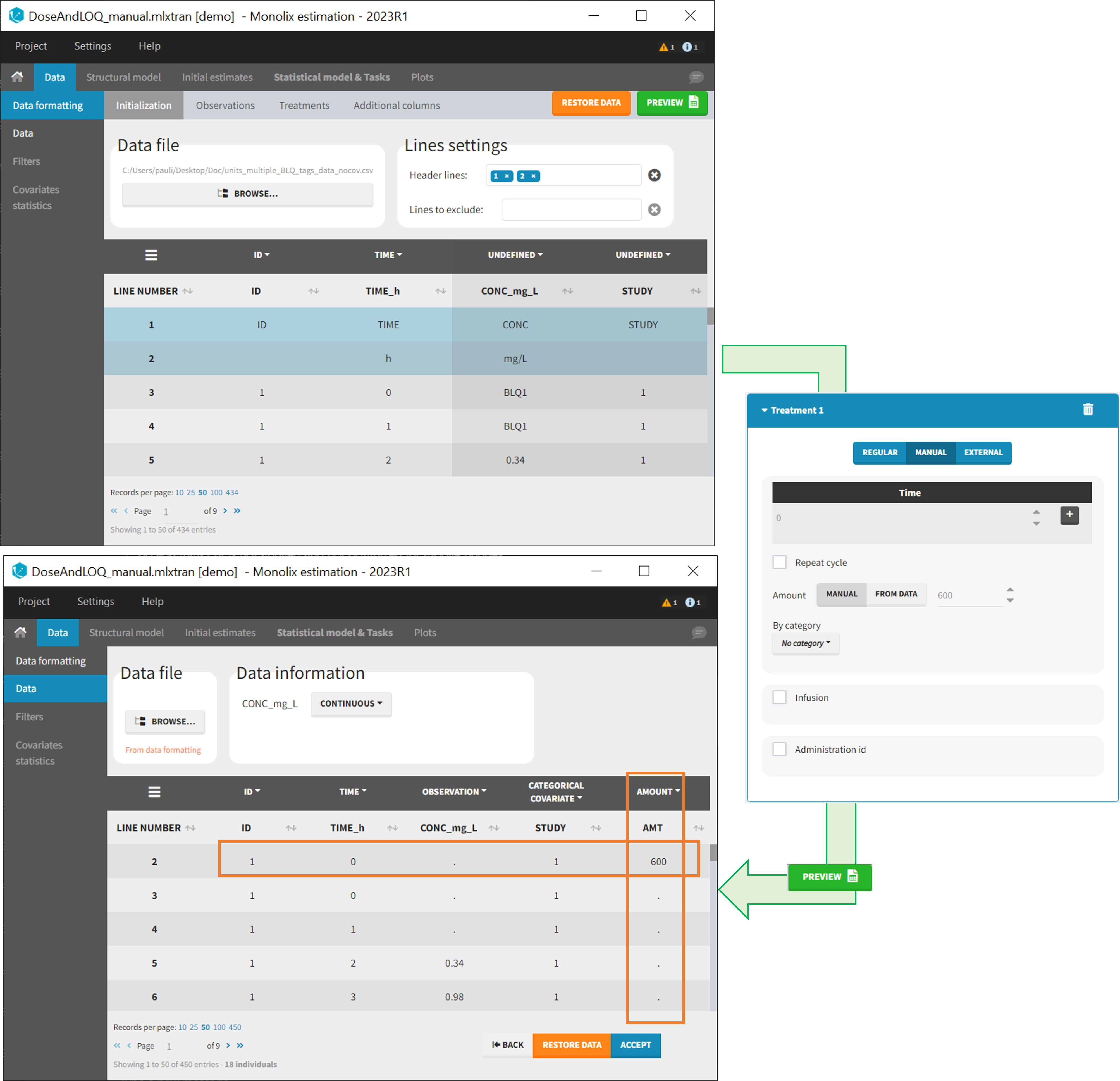
7. Adding doses in the dataset
Datasets in MonolixSuite-standard format should contain all information on doses, as dose lines. An AMOUNT column records the amount of the administrated doses on dose-lines, with “.” on response-lines. In case of infusion, an INFUSION DURATION or INFUSION RATE column records the infusion duration or rate. If there are several types of administration, an ADMINISTRATION ID column can distinguish the different types of doses with integers.
If doses are missing from a dataset, the Data Formatting module can be used to add dose lines and dose-related columns: after initializing the dataset, the user can specify one or several treatments in the Treatments subtab. The following operations are then performed by Data Formatting:
- a new dose line is inserted in the dataset for each defined dose, with the dataset sorted by subject and times. On such a dose line, the values from the next line are duplicated for all columns, except for the observation column in which “.” is used for the dose line.
- A new column AMT is created with “.” on all lines except on dose lines, on which dose amounts are used. The AMT column is automatically tagged as AMOUNT in the Data tab.
- If administration ids have been defined in the treatment, an ADMID column is created, with “.” on all lines except on dose lines, on which administration ids are used. The ADMID column is automatically tagged as ADMINISTRATION ID in the Data tab.
- If an infusion duration or rate has been defined, a new INFDUR (for infusion duration) or INFRATE (for infusion rate) is created, with “.” on all lines except on dose lines. The INFDUR column is automatically tagged as INFUSION DURATION in the Data tab, and the INFRATE column is automatically tagged as INFUSION RATE.
Starting from the 2024R1 version, different dosing schedules can be defined for different individuals, based on information from other columns, which can be useful in cases when different cohorts received different dosing regimens, or when working with data pooled from multiple studies. To define a treatment just for a specific cohort or study, the dropdown on the top of the treatment section can be used:

For each treatment, the dosing schedule can defined as:
- regular: for regularly spaced dosing times, defined with the start time, inter-dose internal, and number of doses. A “repeat cycle” option allows to repeat the regular dosing schedule to generate a more complex regimen.
- manual: a vector of one or several dosing times, each defined manually. A “repeat cycle” option allows to repeat the manual dosing schedule to generate a more complex regimen.
- external: an external text file with columns id (optional), occasions (optional), time (mandatory), amount (mandatory), admid (administration id, optional), tinf or rate (optional), that allows to define individual doses.
While dose amounts, administration ids and infusion durations or rates are defined in the external file for external treatments, available options to define them for treatments of type “manual” or “regular” are:
- “Manual“: this applies the same amount (or administration id or infusion duration or rate) to all doses.
- “By category“: dose amounts (or administration id or infusion duration or rate) are defined manually for different categories read from the dataset.
- “From data“: dose amounts (or administration id or infusion duration or rate) are directly read from the dataset.
The options “by category” and “from data” are described in detail in Section 8.
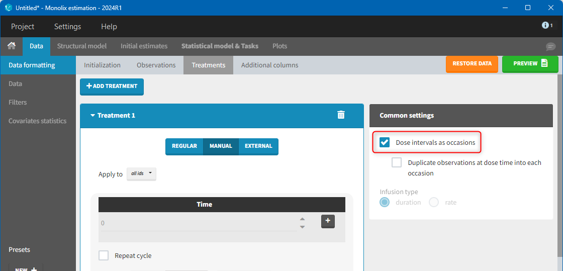
There is a “common settings” panel on the right:
- dose intervals as occasions: this creates a column to distinguish the dose intervals as different occasions (see Section 9).
- infusion type: If several treatments correspond to infusion administration, they need to share the same type of encoding for infusion information: as infusion duration or as infusion rate.
Example:
- demo DoseAndLOQ_manual.mlxtran (the screenshot below focuses on the formatting of doses and excludes other elements present in the demo):
In this demo, doses are initially not included in the dataset to format. A single dose at time 0 with an amount of 600 is added for each individual by Data Formatting. This creates a new AMT column in the formatted dataset, tagged as AMOUNT.
8. Reading censoring limits or dosing information from the dataset
When defining censoring limits for observations (see Section 6) or dose amounts, administration ids, infusion duration or rate for treatments (see Section 7), two options allow to define different values for different rows, based on information already present in the dataset: “by category” and “from data”.
By category
It is possible to define manually different censoring limits, dose amounts, administration ids, infusion durations, or rates for different categories within a dataset’s column. After selecting this column in the “By category” drop-down menu, the different modalities in the column are displayed and a value must be manually assigned each modality.
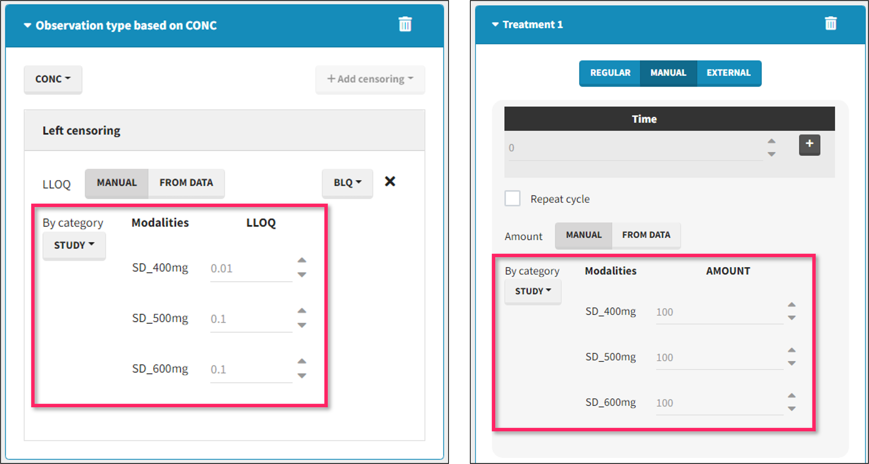
- For censoring limits, the censoring limit used to replace each censoring tag depends on the modality on the same row.
- For doses, the value chosen for the newly created column (AMT for amount, ADMID for administration id, INFDUR for infusion duration, INFRATE for infusion rate) on each new dose line depends on the modality on the first row found in the dataset for the same individual and the same time as the dose, or the next time if there is no line in the initial dataset at that time, or the previous time if no time is found after the dose.
Example:
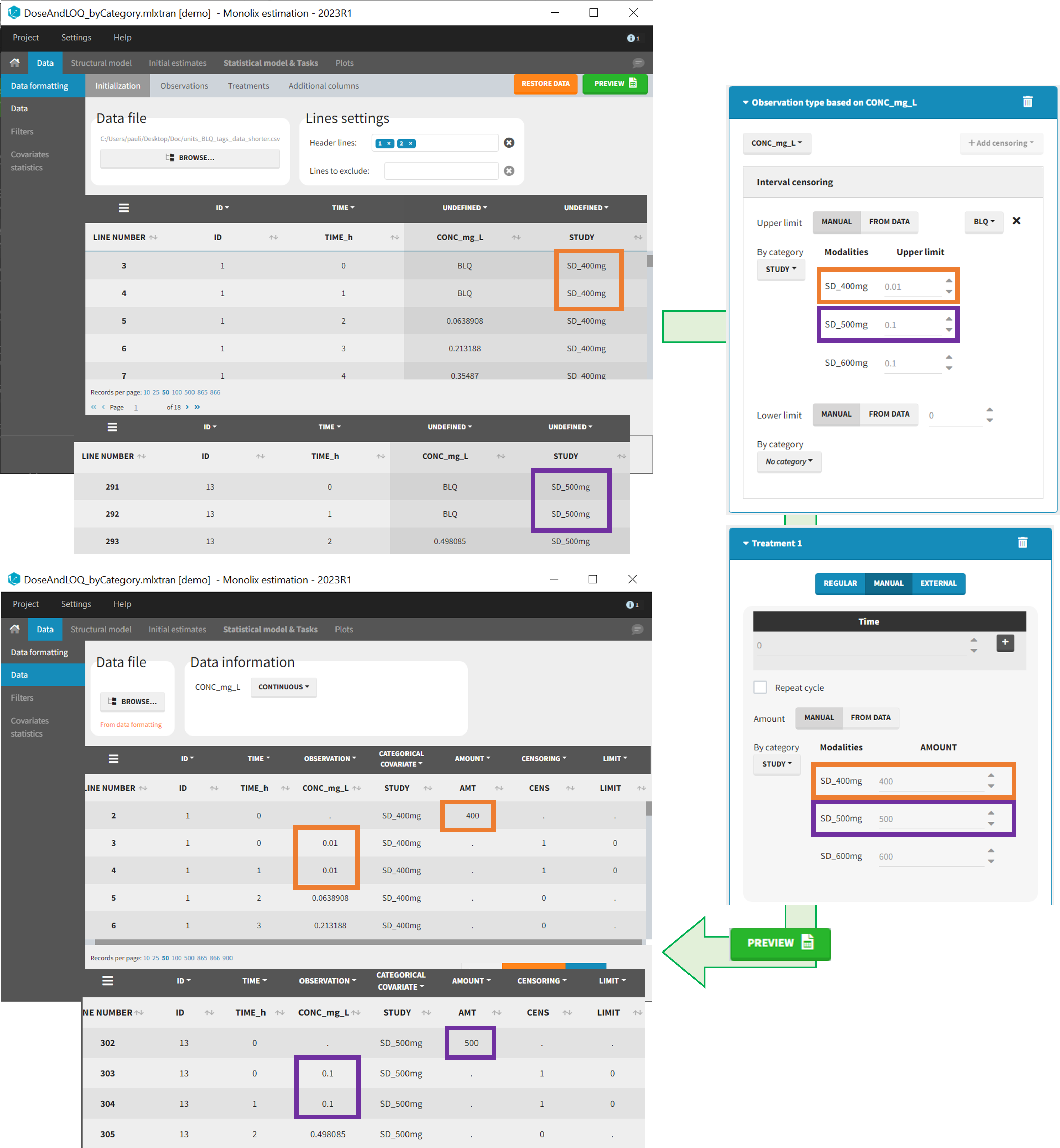
- demo DoseAndLOQ_byCategory.mlxtran (the screenshot below focuses on the formatting of doses and excludes other elements present in the demo):
In this demo there are three studies distinguished in the STUDY column with the categories “SD_400mg”, “SD_500mg” and “SD_600mg”. In Data Formatting, a single dose is manually defined at time 0 for all individuals, with different amounts depending the STUDY category. In addition, censoring interval is defined for the censoring tags BLQ, with an upper limit of the censoring interval (lower limit of quantification) that also depends on the STUDY category. Three new columns – AMT for dose amounts, CENS for censoring tags (0 or 1), and LIMIT for the lower limit of the censoring intervals – are created by Data Formatting. A new dose line is then inserted at time 0 for each individual.
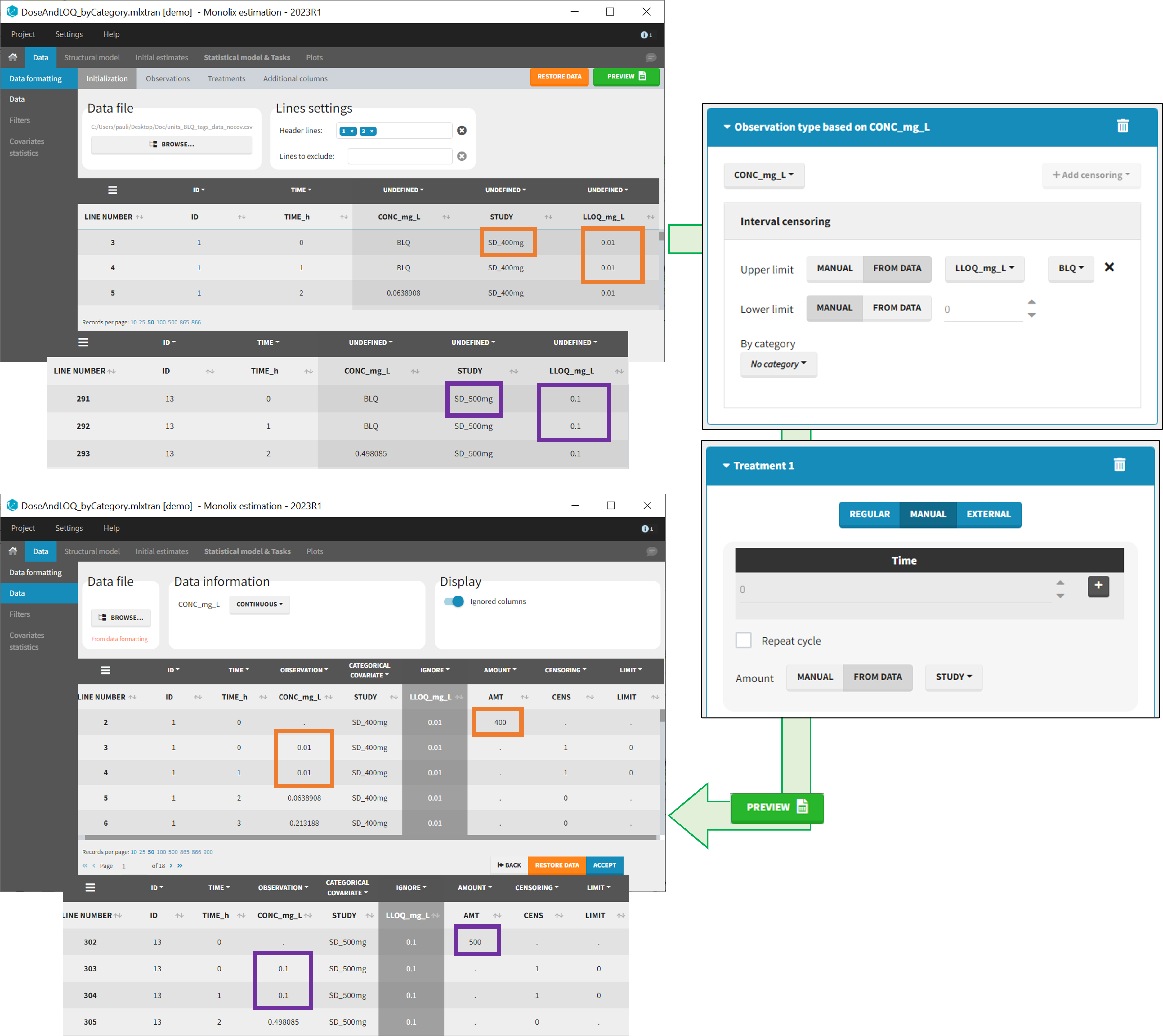
From data
The option “From data” is used to directly read censoring limits, dose amounts, administration ids, infusion durations, or rates from a dataset’s column. The column must contain either numbers or numbers inside strings. In that case, the first number found in the string is extracted (including decimals with .).
- For censoring limits, the censoring limit used to replace each censoring tag is read from the selected column on the same row.
- For doses, the value chosen for the newly created column (AMT for amount, ADMID for administration id, INFDUR for infusion duration, INFRATE for infusion rate) on each new dose line is read from the selected column on the first row found in the dataset for the same individual and the same time as the dose, or the next time if there is no line in the initial dataset at that time, or the previous time if no time is found after the dose.
Example:
- demo DoseAndLOQ_fromData.mlxtran (the screenshot below focuses on the formatting of doses and censoring and excludes other elements present in the demo):
In this demo there are three studies distinguished in the STUDY column with the categories “SD_400mg”, “SD_500mg” and “SD_600mg”. In Data Formatting, a single dose is manually defined at time 0 for all individuals, with the amount read the STUDY column. In addition, censoring interval is defined for the censoring tags BLQ, with an upper limit of the censoring interval (lower limit of quantification) read from the LLOQ_mg_L column. Three new columns – AMT for dose amounts, CENS for censoring tags (0 or 1), and LIMIT for the lower limit of the censoring intervals – are created by Data Formatting. A new dose line is then inserted at time 0 for each individual, with amount 400, 500 or 600 for studies SD_400mg, SD_500mg and SD_600mg respectively.
9. Creating occasions from dosing intervals
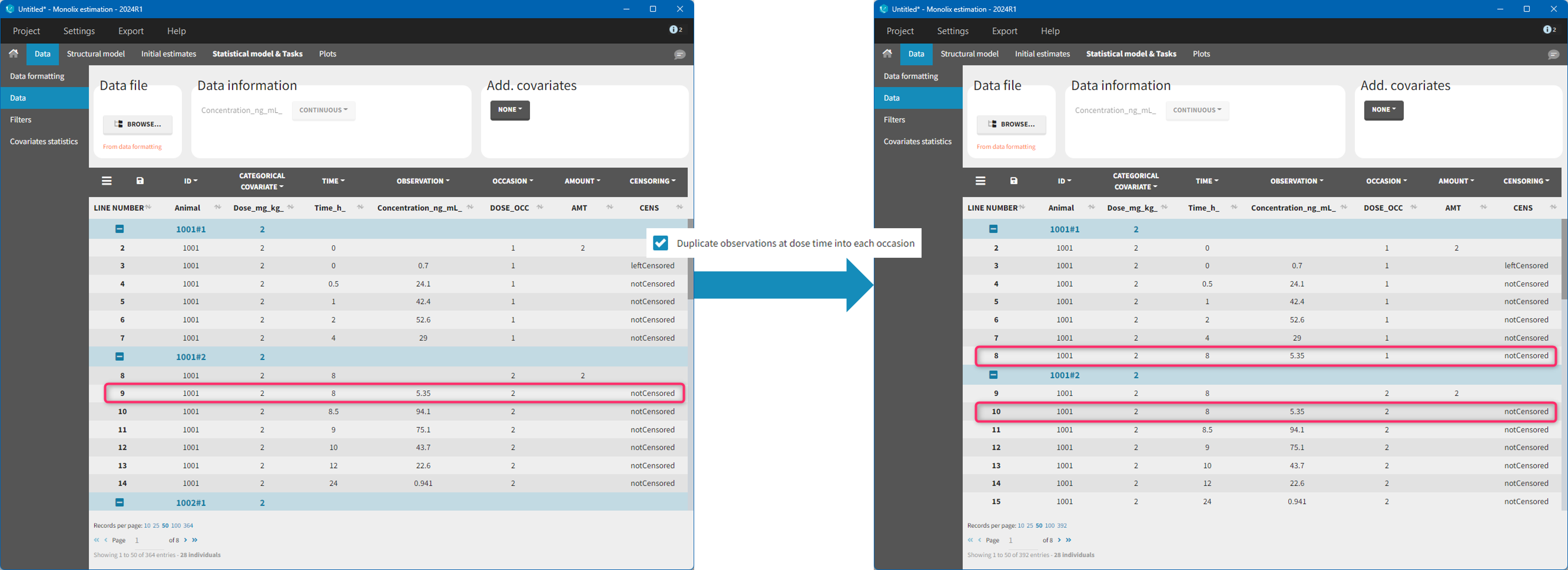
The option “Dose intervals as occasions” in the Treatments subtab of Data Formatting allows to create an occasion column to distinguish dose intervals. This is useful if the sets of measurements following different doses should be analyzed independently for a same individual. From the 2024 version on, an additional option “Duplicate observations at dose times into each occasion” is available. This option allows to duplicate the observations which are at exactly the same time as dose, such that they appear both as last point of the previous occasion and first point of the next occasion. This setting is recommended for NCA, but not recommended for population PK modeling.
Example:
- demo doseIntervals_as_Occ.mlxtran (Monolix demo in the folder 0.data_formatting, here imported into Monolix):
This demo imported from a Monolix demo has an initial dataset in Monolix-standard format, with multiple doses encoded as dose lines with dose amounts in the AMT column. When using this dataset directly into Monolix or Monolix, a single analysis is done on each individual concentration profile considering all doses, which means that NCA would be done on the concentrations after the last dose only, and modeling (CA in Monolix or population modeling in Monolix) would be estimated with a single set of parameter values for each individual. If instead we want to run separate analyses on the sets of concentrations following each dose, we need to distinguish them as occasions with a new column added with the Data Formatting module. To this end, we define the same treatment as in the initial dataset with Data Formatting (here as regular multiple doses) with the option “Dose intervals as occasions” selected. After clicking Preview, Data Formatting adds two new columns: an AMT1 column with the new doses, to be tagged as AMOUNT instead of the AMT column that will now be ignored, and a DOSE_OCC column to be tagged as OCCASION.

Example:
- demo CreateOcc_duplicateObs.pkx imported to Monolix:
10. Handling urine data
In Monolix-standard format, the start and end times of urine collection intervals must be recorded in a single column, tagged as TIME column-type, where the end time of an interval automatically acts as start time for the next interval (see here for more details). If a dataset contains start and end times in two different columns, they can be merged into a single column by Data Formatting. This is done automatically by tagging these two columns as START and END in the Initialization subtab of Data Formatting (see Section 2). In addition the column containing urine collection volume must be tagged as VOLUME.
Example:
- demo Urine_LOQinObs.pkx (Monolix demo here imported into Monolix):
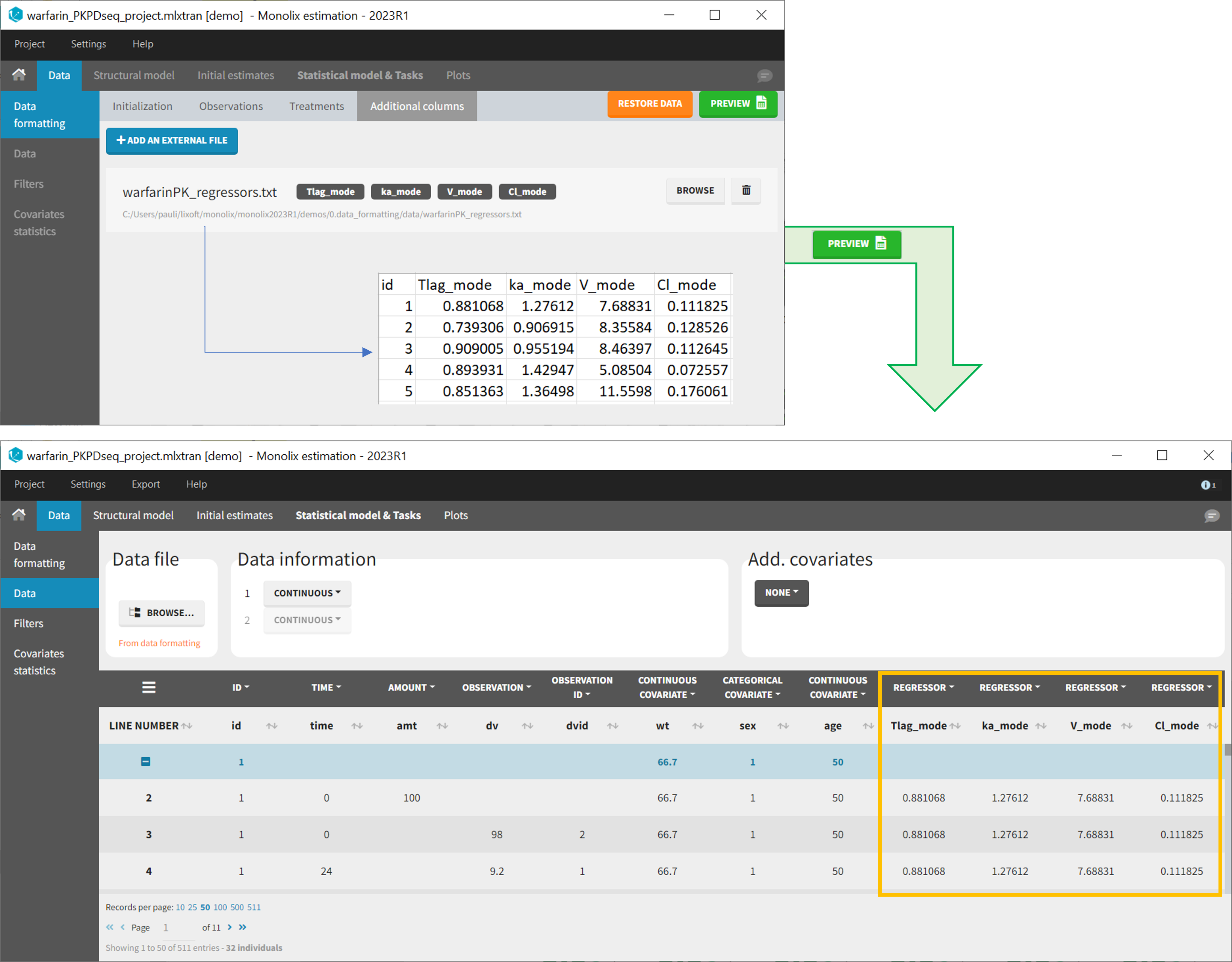
11. Adding new columns from an external file
The last subtab is used to insert additional columns in the dataset from a separate file. The external file must contain a table with a column named ID or id with the same subject identifiers as in the dataset to format, and other columns with a header name and individual values (numbers or strings). There can be only one value per individual, which means that the additional columns inserted in the formatted dataset can contain only a constant value within each individual, and not time-varying values.
Examples of additional columns that can be added with this option are:
- individual parameters estimated in a previous analysis, to be read as regressors to avoid estimating them. Time-varying regressors are not handled.
- new covariates.
If occasions are defined in the formatted dataset, it is possible to have an occasion column in the external file and values defined per subject-occasion.
Example:
- demo warfarin_PKPDseq_project.mlxtran (Monolix demo in the folder 0.data_formatting, here imported into Monolix):
This demo imported from a Monolix demo has an initial PKPD dataset in Monolix-standard format. The option “Additional columns” is used to add the PK parameters estimated on the PK part of the data in another Monolix project.
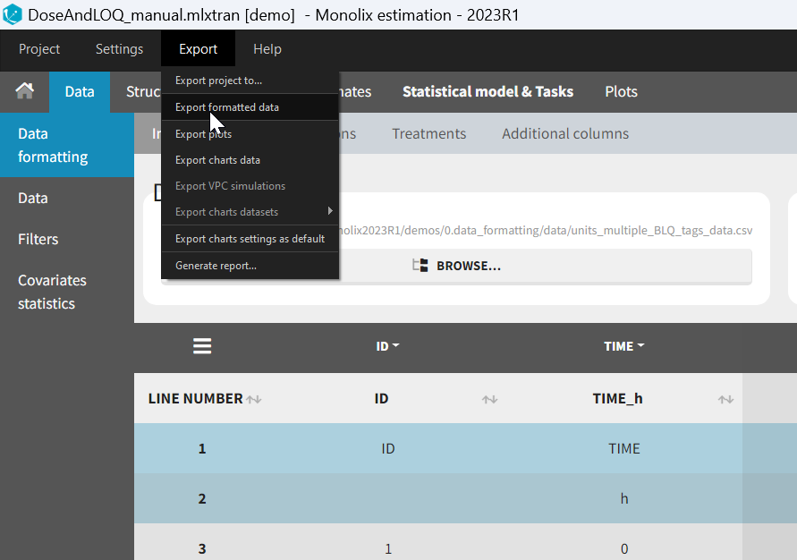
12. Exporting the formatted dataset
Once data formatting is done and the new dataset is accepted, the project can be saved and it is possible to export the formatted dataset as a csv file from the main menu Export > Export formatted data.
2.3.1.Data formatting presets
- Data formatting steps are performed on a specific project.
- Steps are saved in a data formatting preset.
- Preset is reapplied on multiple new projects (manually or automatically).
Creating a data formatting preset
After data formatting steps are done on a project, a preset can be created by clicking on the New button in the bottom left corner of the interface, while in the Data formatting tab: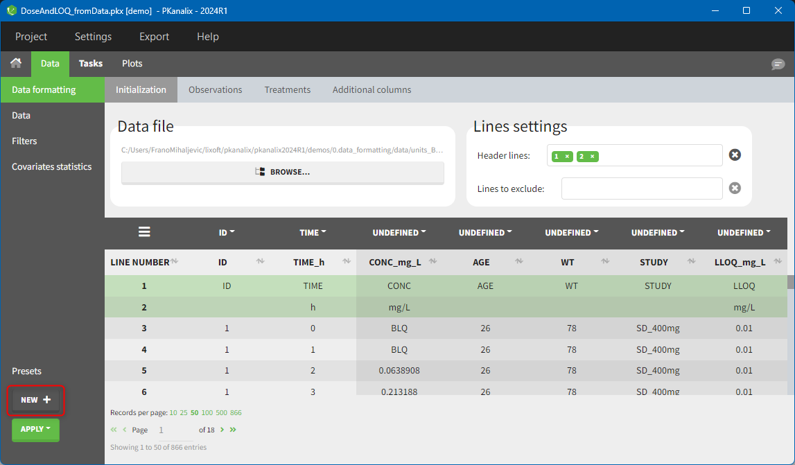
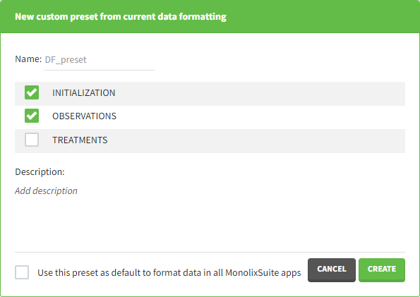
- Name: contains a name of the preset, this information will be used to distinguish between presets when applying them.
- Configuration: contains three checkboxes (initialization, observations, treatments). Users can choose which steps of data formatting will be saved in the preset. If option “External” was used in creating treatments, the external file paths will not be saved in the preset.
- Description: a custom description can be added.
- Use this preset as default to format data in all MonolixSuite apps: if ticked, the preset will be automatically applied every time a data set is loaded for data formatting in PKanalix and Monolix.
Applying a preset
A preset can be applied manually using the Apply button in the bottom left corner of the data formatting tab. Clicking on the Apply button will open a dropdown selection of all saved presets and the desired preset can be chosen. The Apply button is enabled only after the initialization step is performed (ID and TIME columns are selected and the button Next was clicked). This allows PKanalix to fall back to the initialized state, if the initialization step from a preset fails (e.g., if ID and TIME column header saved in the presets do not exist in the new data set). After applying a preset, all data formatting steps saved in the preset will try to be applied. If it is not possible to apply certain steps (e.g., some censoring tags or column headers saved in a preset do not exist), the error message will appear.Managing presets
Presets can be created, deleted, edited, imported and exported by clicking on Settings > Manage Presets > Data Formatting.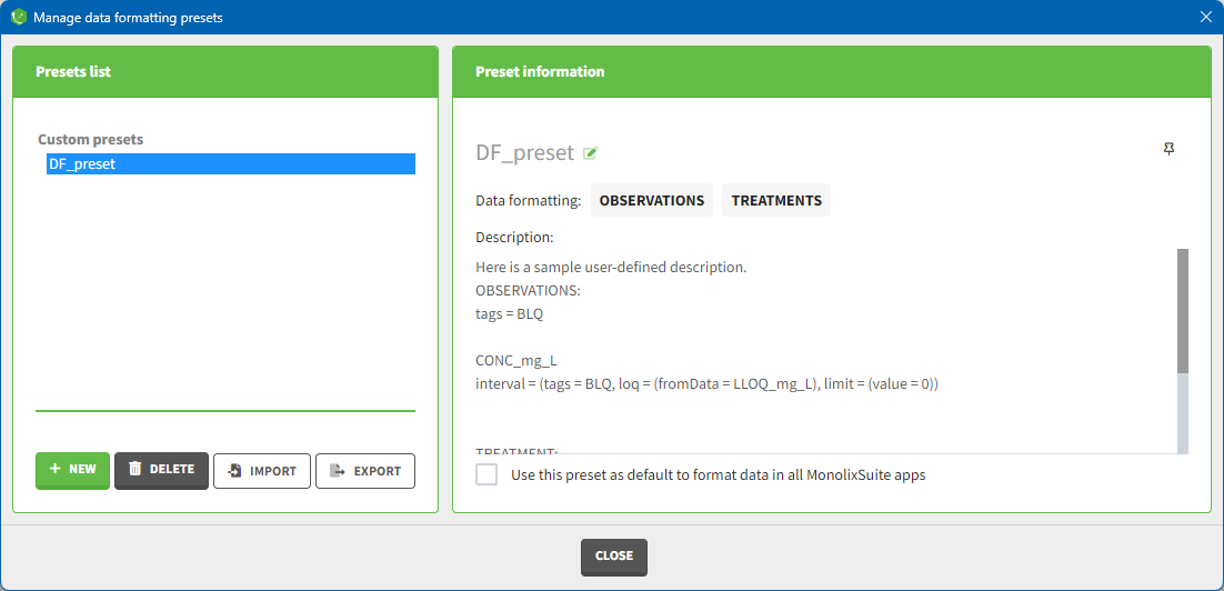
- Create presets: clicking on the button New has the same behavior as clicking on the button New in the Data formatting tab (described in the section “Creating a data formatting preset”).
- Delete presets: clicking on the button Delete will permanently delete a preset. Clicking on this button will not ask for confirmation.
- Edit presets: by clicking on a preset in the left panel, the preset information will appear in the right panel. Name and preset description of the presets can then be updated, and a preset can be selected to automatically format data in PKanalix and Monolix.
- Export presets: a selected preset can be exported as a lixpst file which can be shared between users and imported using the Import button.
- Import presets: a user can import a preset from a lixpst file exported from another computer.
2.4.Filtering a data set
Starting on the 2020 version, it is possible to filter your data set to only take a subpart into account in your modelization. It allows to make filters on some specific IDs, times, measurement values,… It is also possible to define complementary filters and also filters of filters. It is accessible through the filters item on the data tab.
- Creation of a filter
- Filtering actions
- Filters with several actions
- Other filers: filter of filter and complementary filters
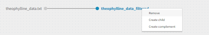
Creation of a filter
To create a filter, you need to click on the data set name. You can then create a “child”. It corresponds to a subpart of the data set where you will define your filtering actions.
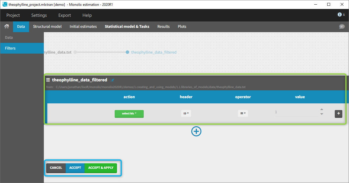
You can see on the top (in the green rectangle) the action that you will complete and you can CANCEL, ACCEPT, or ACCEPT & APPLY with the bottoms on the bottom.
Filtering actions
In all the filtering actions, you need to define
- An action: it corresponds to one of the following possibilities: select ids, remove ids, select lines, remove lines.
- A header: it corresponds to the column of the data set you wish to have an action on. Notice that it corresponds to a column of the data set that was tagged with a header.
- An operator: it corresponds to the operator of choice (=, ≠, < ≤, >, or ≥).
- A value. When the header contains numerical values, the user can define it. When the header contains strings, a list is proposed.
For example, you can
- Remove the ID 1 from your study:

In that case, all the IDs except ID = 1 will be used for the study. - Select all the lines where the time is less or equal 24:

In that case, all lines with time strictly greater that 24 will be removed. If a subject has no measurement anymore, it will be removed from the study. - Select all the ids where SEX equals F:

In that case, all the male will be removed of the study. - Remove all Ids where WEIGHT less or equal 65:

In that case, only the subjects with a weight over 65 will be kept for the study.
In any case, the interpreted filter data set will be displayed in the data tab.
Filters with several actions
In the previous examples, we only did one action. It is also possible to do several actions to define a filter. We have the possibility to define UNION and/or INTERSECTION of actions.
INTERSECTION
By clicking by the + and – button on the right, you can define an intersection of actions. For example, by clicking on the +, you can define a filter corresponding to intersection of
- The IDs that are different to 1.
- The lines with the time values less than 24.

Thus in that case, all the lines with a time less than 24 and corresponding to an ID different than 1 will be used in the study. If we look at the following data set as an example
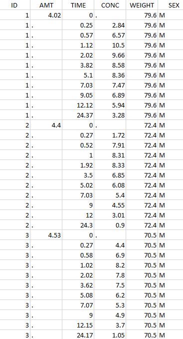 Initial data set |
 Resulting data set after action: select IDs ≠ 1 Resulting data set after action: select IDs ≠ 1 |
 Considered data set for the study as the intersection of the two actions |
 Resulting data set after action: select lines with time ≤ 24 Resulting data set after action: select lines with time ≤ 24 |
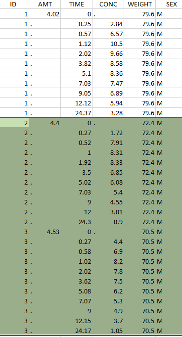
UNION
By clicking by the + and – button on the bottom, you can define an union of actions. For example, in a data set with a multi dose, I can focus on the first and the last dose. Thus, by clicking on the +, you can define a filter corresponding to union of
- The lines where the time is strictly less than 12.
- The lines where the time is greater than 72.

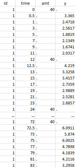 Initial data set |
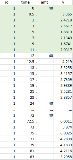 Resulting data set after action: select lines where the time is strictly less than 12 |
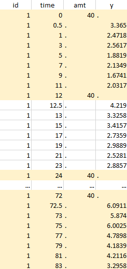 Considered data set for the study as the union of the three actions |
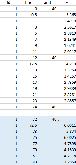 Resulting data set after action: select lines where the time is greater than 72 |
||
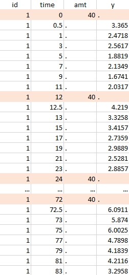 Resulting data set after action: select lines where amt equals 40 |
Notice that, if just define the first two actions, all the dose lines at a time in ]12, 72[ will also be removed. Thus, to keep having all the doses, we need to add the condition of selecting the lines where the dose is defined.
In addition, it is possible to do any combination of INTERSECTION and UNION.
Other filers: filter of filter and complementary filters
Based on the definition of a filter, it is possible to define two other actions. By clicking on the filter, it is possible to create
- A child: it corresponds to a new filter with the initial filter as the source data set.
- A complement: corresponds to the complement of the filter. For example, if you defined a filter with only the IDs where the SEX is F, then the complement corresponds to the IDs where the SEX is not F.
2.5.Handling censored (BLQ) data
- Introduction
- Theory
- Censoring definition in a data set
- PK data below a lower limit of quantification
- PK data below a lower limit of quantification or below a limit of detection
- PK data below a lower limit of quantification and PD data above an upper limit of quantification
- Combination of interval censored PK and PD data
- Case studies
Objectives: learn how to handle easily and properly censored data, i.e. data below (resp. above) a lower (resp.upper) limit of quantification (LOQ) or below a limit of detection (LOD).
Projects: censoring1log_project, censoring1_project, censoring2_project, censoring3_project, censoring4_project
Introduction
Censoring occurs when the value of a measurement or observation is only partially known. For continuous data measurements in the longitudinal context, censoring refers to the values of the measurements, not the times at which they were taken. For example, the lower limit of detection (LLOD) is the lowest quantity of a substance that can be distinguished from its absence. Therefore, any time the quantity is below the LLOD, the “observation” is not a measurement but the information that the measured quantity is less than the LLOD. Similarly, in longitudinal studies of viral kinetics, measurements of the viral load below a certain limit, referred to as the lower limit of quantification (LLOQ), are so low that their reliability is considered suspect. A measuring device can also have an upper limit of quantification (ULOQ) such that any value above this limit cannot be measured and reported.
As hinted above, censored values are not typically reported as a number, but their existence is known, as well as the type of censoring. Thus, the observation }_{ij}")

We usually distinguish between three types of censoring: left, right and interval. In each case, the SAEM algorithm implemented in Monolix properly computes the maximum likelihood estimate of the population parameters, combining all the information provided by censored and non censored data.
Theory
In the presence of censored data, the conditional density function needs to be computed carefully. To cover all three types of censoring (left, right, interval), let 

$$\displaystyle p(y^{(r)}|\psi)=\prod_{i=1}^{N}\prod_{j=1}^{n_i}p(y_{ij}|\psi_i)^{1_{y_{ij}\notin I_{ij}}}\mathbb{P}(y_{ij}\in I_{ij}|\psi_i)^{1_{y_{ij}\in I_{ij}}}$$
where
$$\displaystyle \mathbb{P}(y_{ij}\in I_{ij}|\psi_i)=\int_{I_{ij}} p_{y_{ij}|\psi_i} (u|\psi_i)du$$
We see that if 
")
")
For the calculation of the likelihood, this is equivalent to the M3 method in NONMEM when only the CENSORING column is given, and to the M4 method when both a CENSORING column and a LIMIT column are given.
Censoring definition in a data set
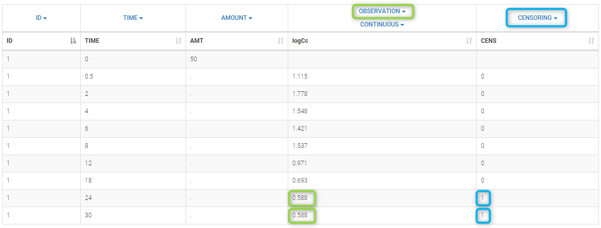
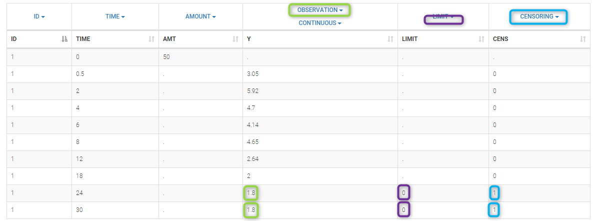
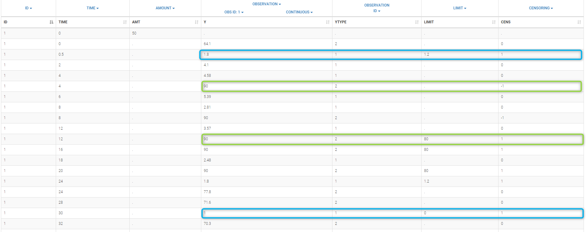
In the dataset format used by Monolix and PKanalix, censored information is included in this way:
- The censored measurement should be in the OBSERVATION column.
- In an additional CENSORING column, put 0 if the observation is not censored, and 1 or – 1 depending if the measurement given in the observation column is a lower or an upper limit.
- Optionally, include a LIMIT column to set the other limit.
To quickly include censoring information to your dataset by using BLQ tags in the observation column, you can use data formatting.
Examples are provided below and here.
PK data below a lower limit of quantification
Left censored data
- censoring1log_project (data = ‘censored1log_data.txt’, model = ‘pklog_model.txt’)
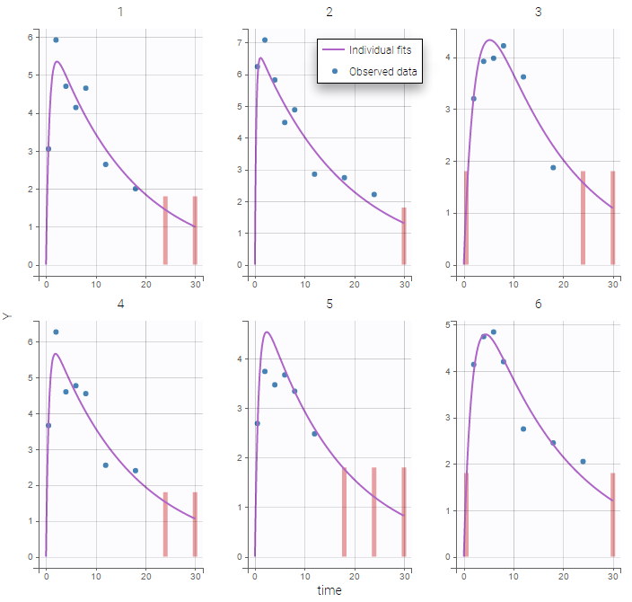
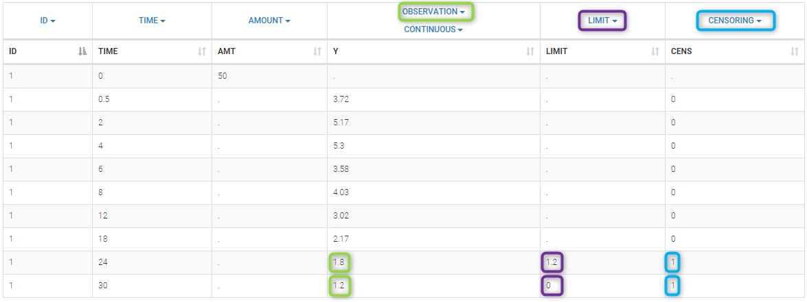
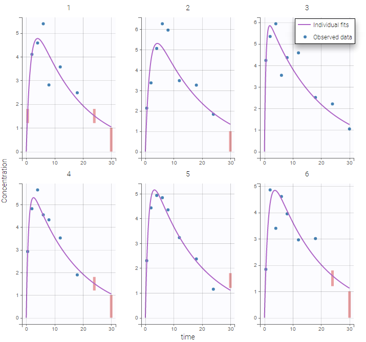
PK data are log-concentration in this example. The limit of quantification of 1.8 mg/l for concentrations becomes log(1.8)=0.588 for log-concentrations. The column of observations (Y) contains either the LLOQ for data below the limit of quantification (BLQ data) or the measured log-concentrations for non BLQ data. Furthermore, Monolix uses an additional column CENSORING to indicate if an observation is left censored (CENS=1) or not (CENS=0). In this example, subject 1 has two BLQ data at times 24h and 30h (the measured log-concentrations were below 0.588 at these times):
The plot of individual fits displays BLQ (red band) and non BLQ data (blue dots) together with the predicted log-concentrations (purple line) on the whole time interval:
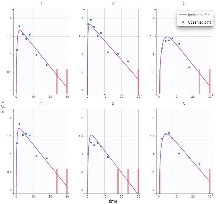
Notice that the band goes from .8 to -Infinity as no bound has been specified (no LIMIT column was proposed).
For diagnosis plots such as VPC, residuals of observations versus predictions, Monolix samples the BLQ data from the conditional distribution
$$p(y^{BLQ} | y^{non BLQ}, \hat{\psi}, \hat{\theta})$$
where 

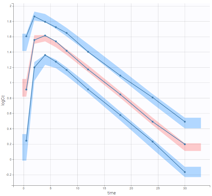
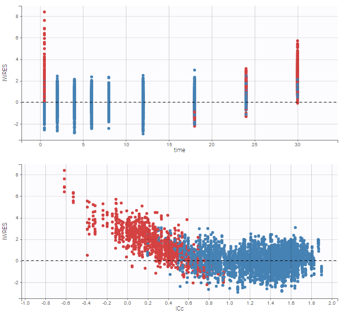
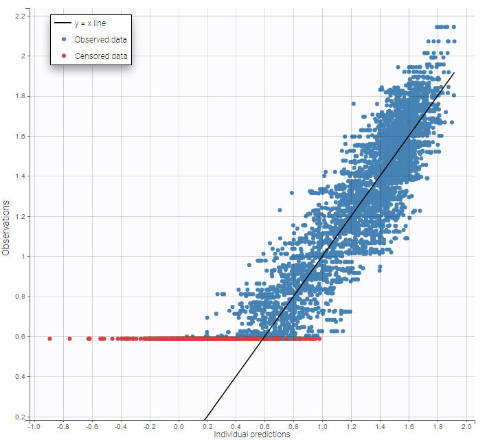
A strong bias appears if LLOQ is used instead for the BLQ data (if you choose LOQ instead of simulated in the display frame of the settings) :
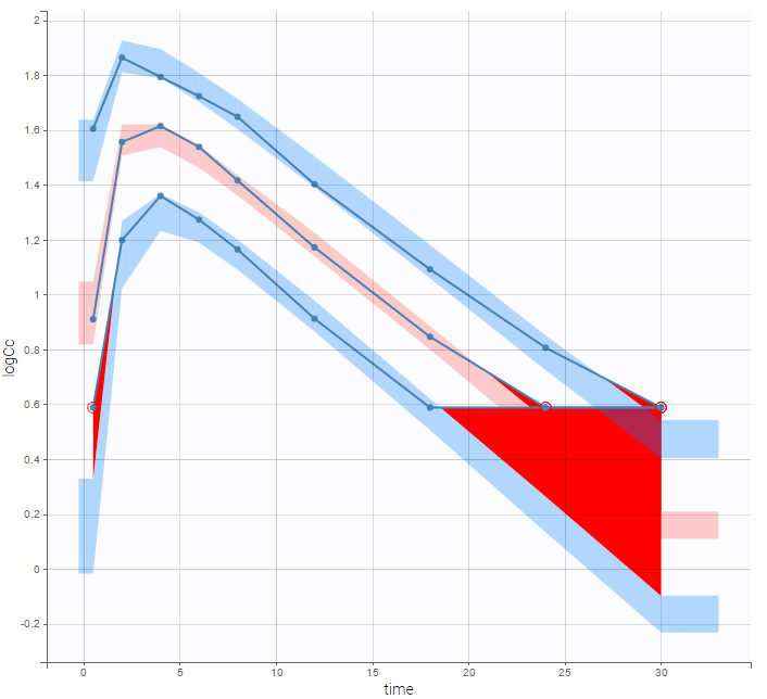
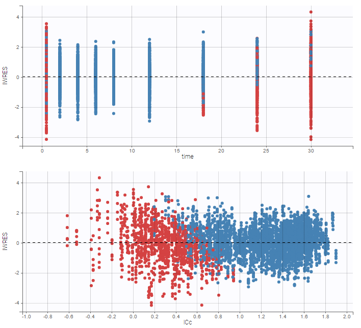
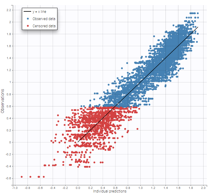
Notice that ignoring the BLQ data entails a loss of information as can be seen below (if you choose no in the “Use BLQ” toggle):
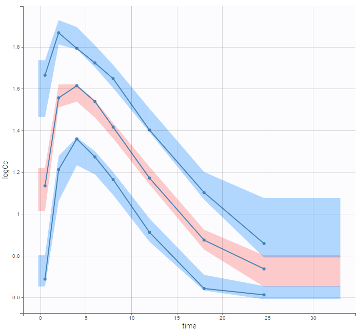
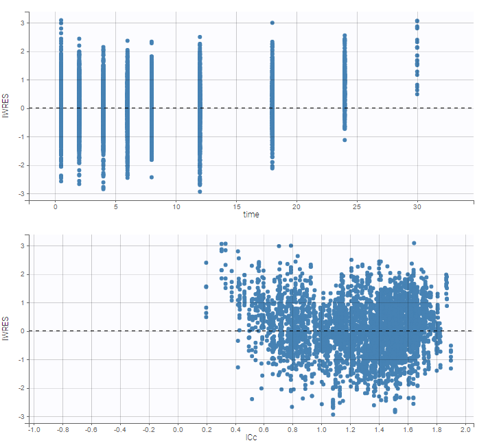
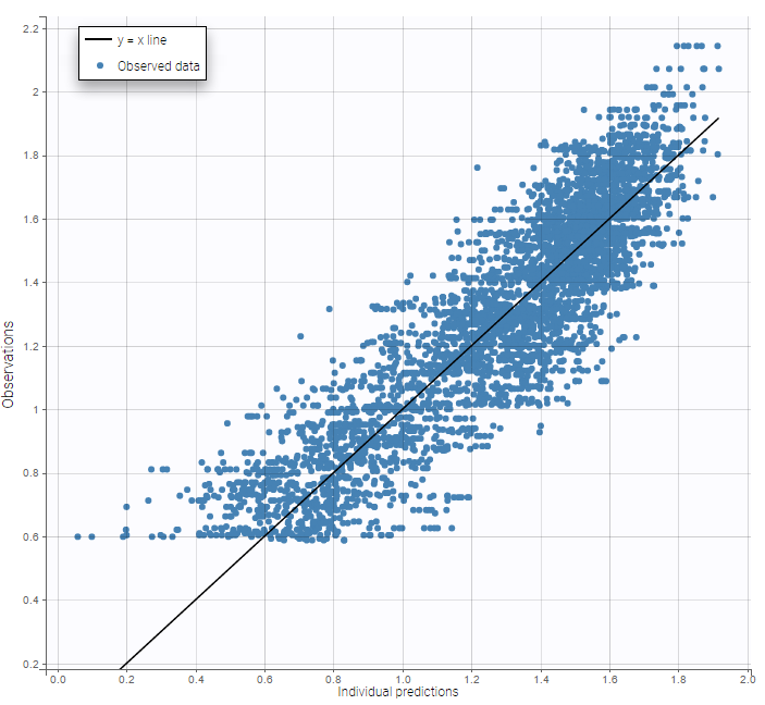
As can be seen below, imputed BLQ data is also used for residuals (IWRES on the left) and for observations versus predictions (on the right)
 |
 |
|---|
More on these diagnosis plots
Impact of the BLQ in residuals and observations versus predictions plots
A strong bias appears if LLOQ is used instead for the BLQ data for these two diagnosis plots:
 |
 |
|---|
while ignoring the BLQ data entails a loss of information:
 |
 |
|---|
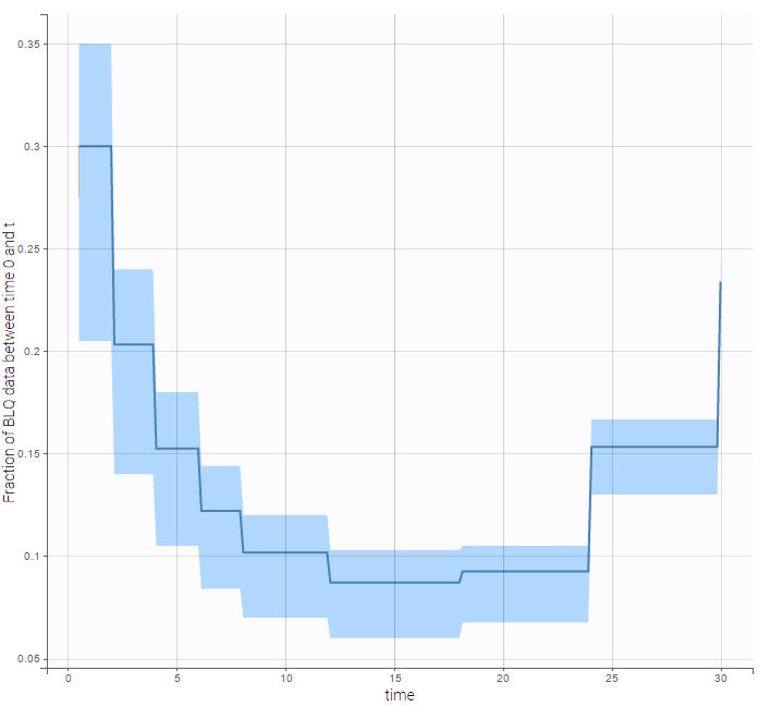
BLQ predictive checks
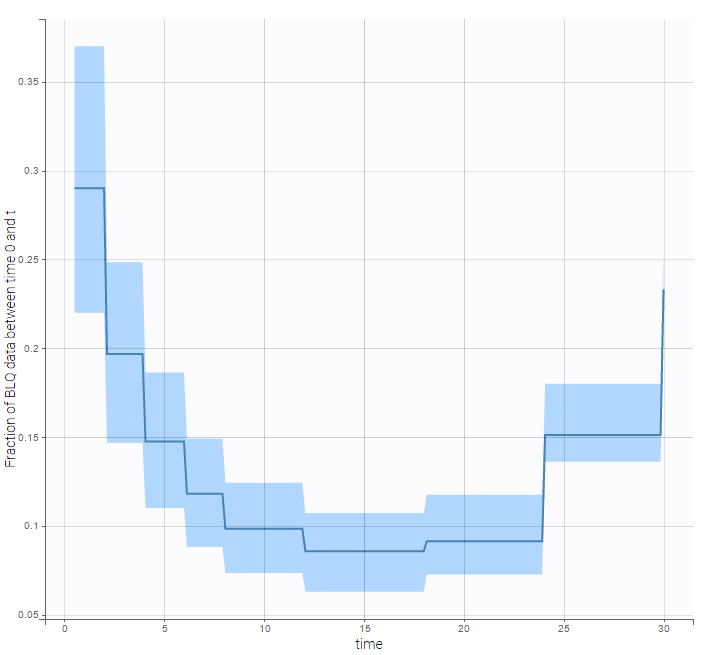
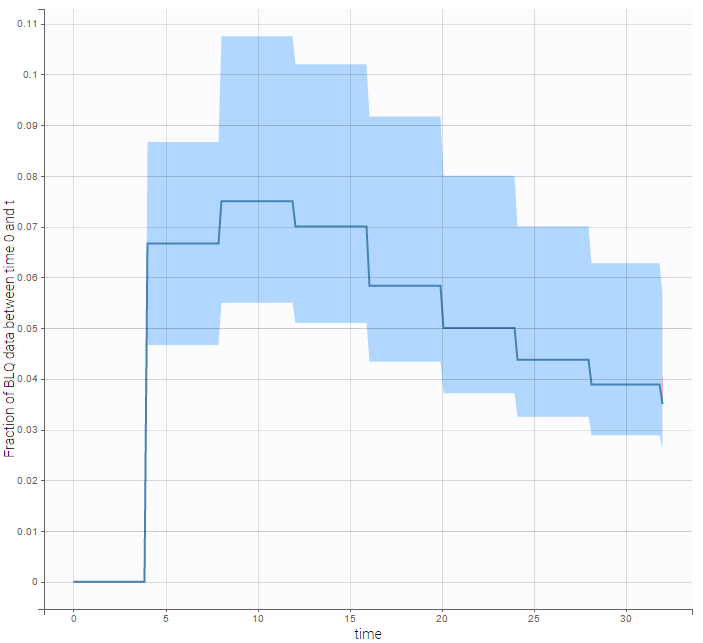
The BLQ predictive check is a diagnosis plot that displays the fraction of cumulative BLQ data (blue line) with a 90% prediction interval (blue area).
Interval censored data
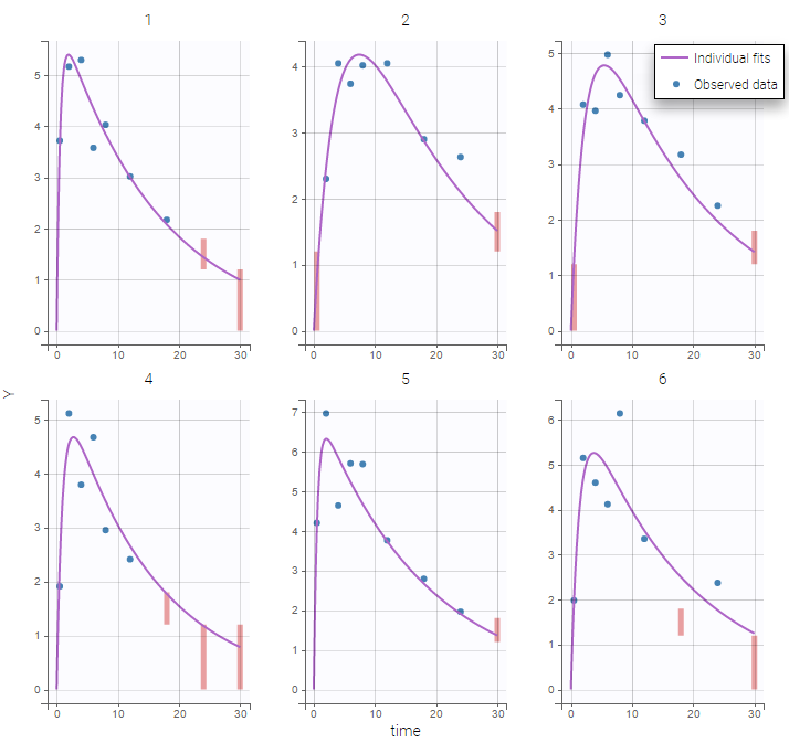
- censoring1_project (data = ‘censored1_data.txt’, model = ‘lib:oral1_1cpt_kaVk.txt’)
We use the original concentrations in this project. Then, BLQ data should be treated as interval censored data since a concentration is know to be positive. In other word, a data reported as BLQ data means that the (non reported) measured concentration is between 0 and 1.8mg/l. The value in the observation column 1.8 indicates the value, the value in the CENSORING column indicates that the value in the observation column is the upper bound. An additional column LIMIT reports the lower limit of the censored interval (0 in this example):
Remarks
- if this column is missing, then BLQ data is assumed to be left-censored data that can take any positive and negative value below LLOQ.
- the value of the limit can vary between observations of the same subject.
Monolix will use this additional information to estimate the model parameters properly and to impute the BLQ data for the diagnosis plots.
Plot of individual fits now displays LLOD at 1.8 with a red band when a PK data is censored. We see that the band lower limit is at 0 as defined in the limit column.
PK data below a lower limit of quantification or below a limit of detection
- censoring2_project (data = ‘censored2_data.txt’, model = ‘lib:oral1_1cpt_kaVk.txt’)
 Plot of individual fits now displays LLOQ or LLOD with a red band when a PK data is censored. We see that the band lower limits depend on the observation.
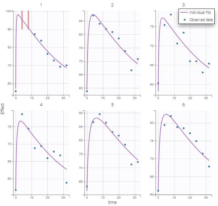
PK data below a lower limit of quantification and PD data above an upper limit of quantification
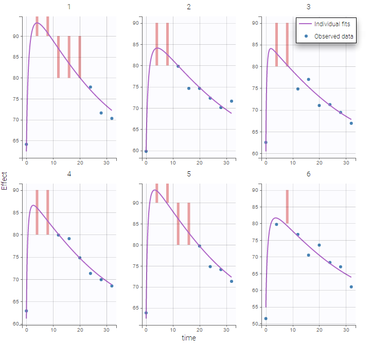
- censoring3_project (data = ‘censored3_data.txt’, model = ‘pkpd_model.txt’)
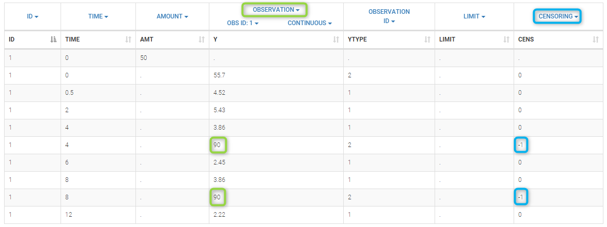
We work with PK and PD data in this project and assume that the PD data may be right censored and that the upper limit of quantification is ULOQ=90. We use CENS=-1 to indicate that an observation is right censored. In such case, the PD data can take any value above the upper limit reported in column Y (here the YTYPE column of type OBSERVED ID defines the type of observation, YTYPE=1 and YTYPE=2 are used respectively for PK and PD data):
 Plot of individual fits for the PD data now displays ULOQ and the predicted PD profile:
We can display the cumulative fraction of censored data both for the PK and the PD data (on the left and right respectively):
 |
 |
|---|
Combination of interval censored PK and PD data
- censoring4_project (data = ‘censored4_data.txt’, model = ‘pkpd_model.txt’)
We assume in this example
- 2 different censoring intervals(0,1) and (1.2, 1.8) for the PK,
- a censoring interval (80,90) and right censoring (>90) for the PD.
Combining columns CENS, LIMIT and Y allow us to combine efficiently these different censoring processes:
This coding of the data means that, for subject 1,
- PK data is between 0 and 1 at time 30h (second blue frame),
- PK data is between 1.2 and 1.8 at times 0.5h and 24h (first blue frame for time .5h),
- PD data is between 80 and 90 at times 12h and 16h (second green frame for time 12h),
- PD data is above 90 at times 4h and 8h (first green frame for time 4h).
Plot of individual fits for the PK and the PD data displays the different limits of these censoring intervals (PK on the left and PD on the right):
 |
 |
|---|
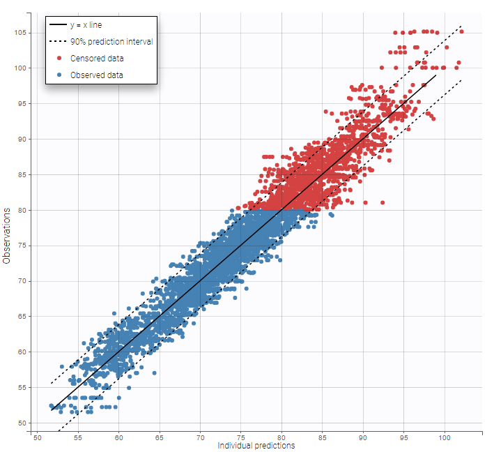
Other diagnosis plots, such as the plot of observations versus predictions, adequately use imputed censored PK and PD data:
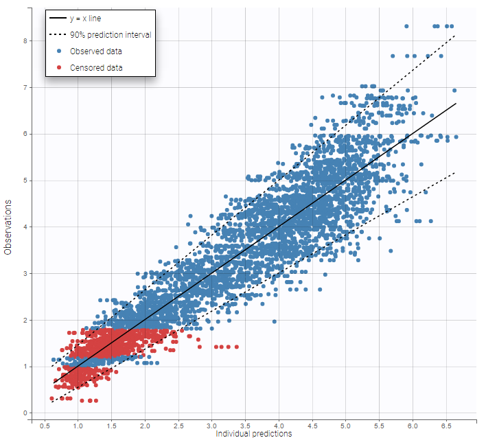 |
 |
|---|
Case studies
- 8.case_studies/hiv_project (data = ‘hiv_data.txt’, model = ‘hivLatent_model.txt’)
- 8.case_studies/hcv_project (data = ‘hcv_data.txt’, model = ‘hcvNeumann98_model_latent.txt’)
2.6.Mapping between the data and the model
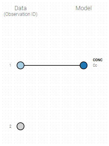
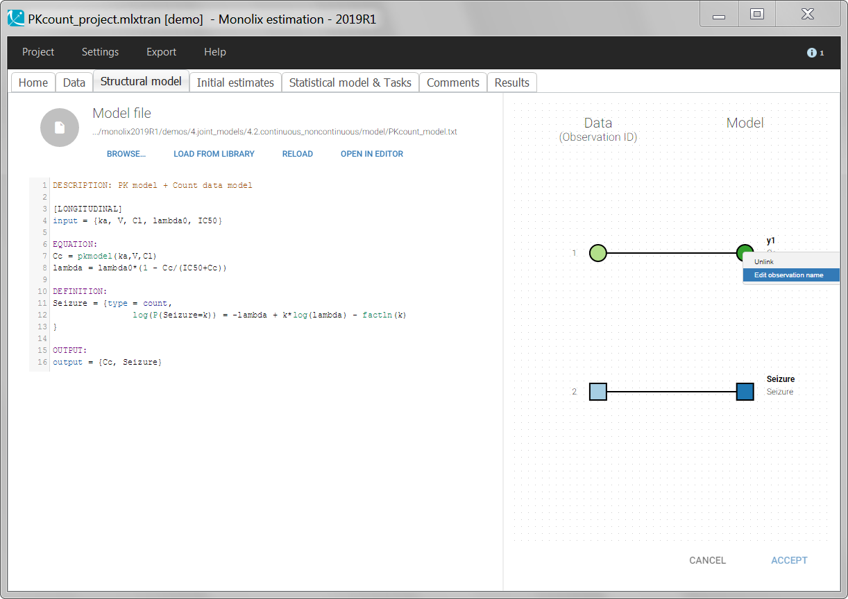
Starting from the 2019 version, it is possible to change the mapping between the data set observations ids and the structural model output. By default and in previous versions, the mapping is done by order, i.e. the first output listed in the output= statement of the model is mapped to the first OBSERVATION ID (ordered alphabetically). It is possible with the interface to set exactly which model output is mapped to which data output. Model output or data outputs can be left unused.
Changing the mapping
If you have more output in the data set (i.e more OBSERVATION IDs) than in the structural model, you can set which data output you will use in the project. In the example below there are two outputs in the data set (managed by the OBSERVATION ID column) and only one output in the structural model, Cc. By default the following mapping is proposed: the data with observation id ‘1’ is mapped to the modle prediction ‘Cc’. The model observation (with error model) is called ‘CONC’ (the name of the OBSERVATION column, can be edited):
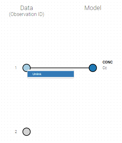
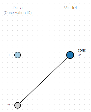
To set the data output to use to observation id ‘2’, you can either:
- Unlink by clicking on either the dot representing the output ‘1’ of the Data or ‘Cc’ of the structural model, and then draw the line between ‘2’ and ‘Cc’ (as can be seen on the figure below on the left)
- Directly draw a line from ‘2’ to ‘Cc’ (as can be seen on the figure below on the right). This will automatically undo the link between ‘1’ and ‘Cc’.
 |
 |
|---|
And click on the button ACCEPT on the bottom on the window to apply the changes.
The same possibility is proposed if you have more outputs in the structural model, compared to the number of observation ids. If you have a TMDD model with both the free and the total ligand concentration listed as model output and one type of measurement, you can map either the free or the total ligand as can be seen on the following figure with the same actions as described above.
Several types of outputs
The mapping is only possible between outputs of same nature (continuous / count-categorical / event), i.e. it is only possible to map a continuous output with a continuous output of the structural model. Thus, mapping a continuous output with a discrete or a time-to-event is not possible. If you try to link a forbidden combination, the line connecting line will be displayed in red as in the following figure
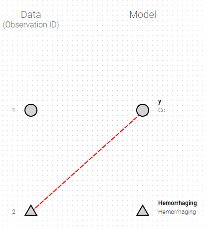
The type of output is indicated via the shapes:
- continuous outputs are displayed as circles
- categorical/count outputs are displayed as squares
- event outputs are displayed as triangles
Changing the observation name
In the example below, ‘1’ is the observation id used in the data set to identify the data to use, ‘Cc’ is the model output (a prediction, without residual error) and ‘y1’ the observation (with error). ‘y1’ represents the data with observation id ‘1’ and it appears in the labels/legends of the plots. These elements are related by observation model, which formula can be displayed.
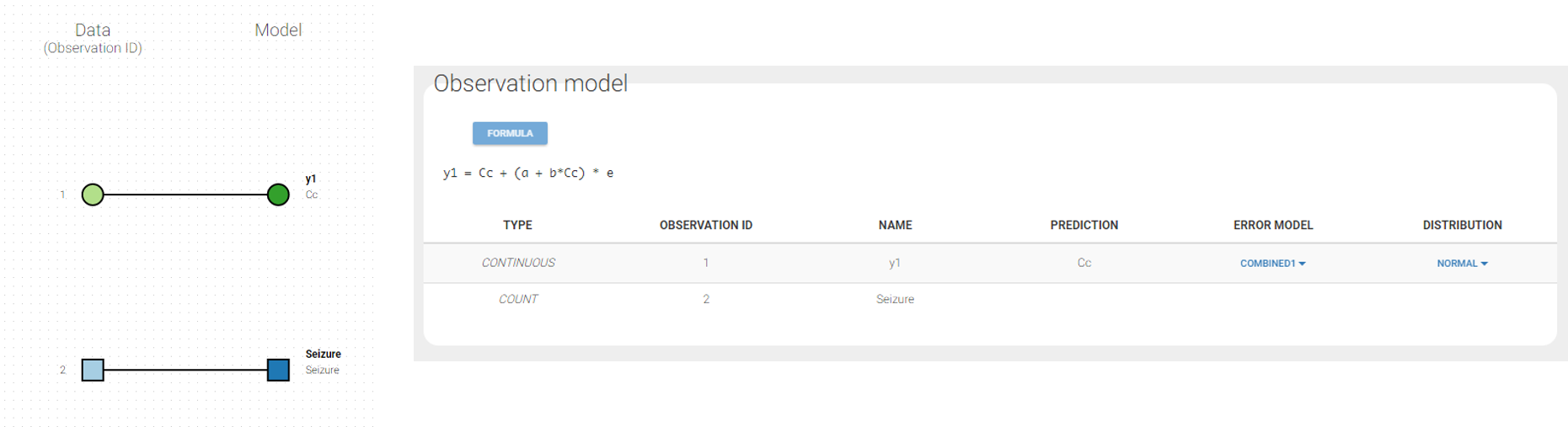
For count/categorical and event model outputs, the model observation is defined in the model file directly. The name used in the model file is reused in the mapping interface and cannot be changed.
For continuous outputs, the model file defines the name of the prediction (e.g ‘Cc’), while the model observation (e.g ‘y1’, with error) definition is done in the “Statistical model and tasks” tab of the interface. If there is only one model output, the default observation name is the header of the data set column tagged as OBSERVATION. In case of several model outputs, the observation names are y1, y2, y3, etc. The observation names for continuous outputs can be changed by clicking on the node and “edit observation name”:
3.Structural model
3.1.Libraries of models
- The PK library
- The PD and PKPD libraries
- The PK double absorption library
- The TMDD library
- The TTE library
- The Count library
- The TGI library
- A step-by-step example with the PK library
Objectives: learn how to use the Monolix libraries of models and use your own models.
Projects: theophylline_project, PDsim_project, warfarinPK_project, TMDD_project, LungCancer_project, hcv_project
For the definition of the structural model, the user can either select a model from the available model libraries or write a model itself using the Mlxtran language.
Discover how to easily choose a model from the libraries via step-by-step selection of its characteristics. An enriched PK, a PD, a joint PKPD, a target-mediated drug disposition (TMDD), and a time to-event (TTE) library are now available.
Model libraries
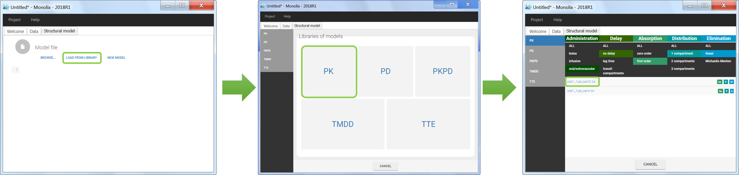
Five different model libraries are available in Monolix, which we will detail below. To use a model from the libraries, in the Structural model tab, click on Load from library and select the desired library. A list of model files appear, as well as a menu to filter them. Use the filters and indications in the file name (parameters names) to select the model file you need.
The model files are simply text files that contain pre-written models in Mlxtran language. Once selected, the model appears in the Monolix GUI. Below we show the content of the (ka,V,Cl) model:
The PK library
- theophylline_project (data = ‘theophylline_data.txt’ , model=’lib:oral1_1cpt_kaVCl.txt’)
The PK library includes model with different administration routes (bolus, infusion, first-order absorption, zero-order absorption, with or without Tlag), different number of compartments (1, 2 or 3 compartments), and different types of eliminations (linear or Michaelis-Menten). More details, including the full equations of each model, can be found on the PK model library wepage. The PK library models can be used with single or multiple doses data, and with two different types of administration in the same data set (oral and bolus for instance).
The PD and PKPD libraries
- PDsim_project (data = ‘PDsim_data.txt’ , model=’lib:immed_Emax_const.txt’)
The PD model library contains direct response models such as Emax and Imax with various baseline models, and turnover response models. These models are PD models only and the drug concentration over time must be defined in the data set and passed as a regressor.
- warfarinPKPD_project (data = ‘warfarin_data.txt’, model = ‘lib:oral1_1cpt_IndirectModelInhibitionKin_TlagkaVClR0koutImaxIC50.txt’)
The PKPD library contains joint PKPD models, which correspond to the combination of the models from the PK and from the PD library. These models contain two outputs, and thus require the definition of two observation identifiers (i.e two different values in the OBSERVATION ID column).
Complete description of the PD and PK/PD model libraries.
The PK double absorption library
The library of double absorption models contains all the combinations for two mixed absorptions, with different types and delays. The absorptions can be specified as simultaneous or sequential, and with a pre-defined or independent order. This library simplifies the selection and testing of different types of absorptions and delays. More details about the library and examples can be found on the dedicated PK double absorption documentation page.
The TMDD library
- TMDD_project (data = ‘TMDD_dataset.csv’ , model=’lib:bolus_2cpt_MM_VVmKmClQV2_outputL.txt’)
The TMDD library contains various models for molecules displaying target-mediated drug disposition (TMDD). It includes models with different administration routes (bolus, infusion, first-order absorption, zero-order absorption, bolus + first-order absorption, with or without Tlag), different number of compartments (1, or 2 compartments), different types of TMDD models (full model, MM approximation, QE/QSS approximation, etc), and different types of output (free ligand or total free+bound ligand). More details about the library and guidelines to choose model can be found on the dedicated TMDD documentation page.
The TTE library
- LungCancer_project (data = ‘lung_cancer_survival.csv’ , model=’lib:gompertz_model_singleEvent.txt’)
The TTE library contains typical parametric models for time-to-event (TTE) data. TTE models are defined via the hazard function, in the library we provide exponential, Weibull, log-logistic, uniform, Gompertz, gamma and generalized gamma models, for data with single (e.g death) and multiple events (e.g seizure) per individual. More details and modeling guidelines can be found on the TTE dedicated webpage, along with case studies.
The Count library
The Count library contains the typical parametric distributions to describe count data. More details can be found on the Count dedicated webpage, with a short introduction on count data, the different ways to model this kind of data, and typical models.
The tumor growth inhibition (TGI) library
A wide range of models for tumour growth (TG) and tumour growth inhibition (TGI) is available in the literature and correspond to different hypotheses on the tumor or treatment dynamics. In MonolixSuite2020, we provide a modular TG/TGI model library that combines sets of frequently used basic models and possible additional features. This library permits to easily test and combine different hypotheses for the tumor growth kinetics and effect of a treatment, allowing to fit a large variety of tumor size data.
Complete description of the TGI model library.
Step-by-step example with the PK library
- theophylline_project (data = ‘theophylline_data.txt’ , model=’lib:oral1_1cpt_kaVCl.txt’)
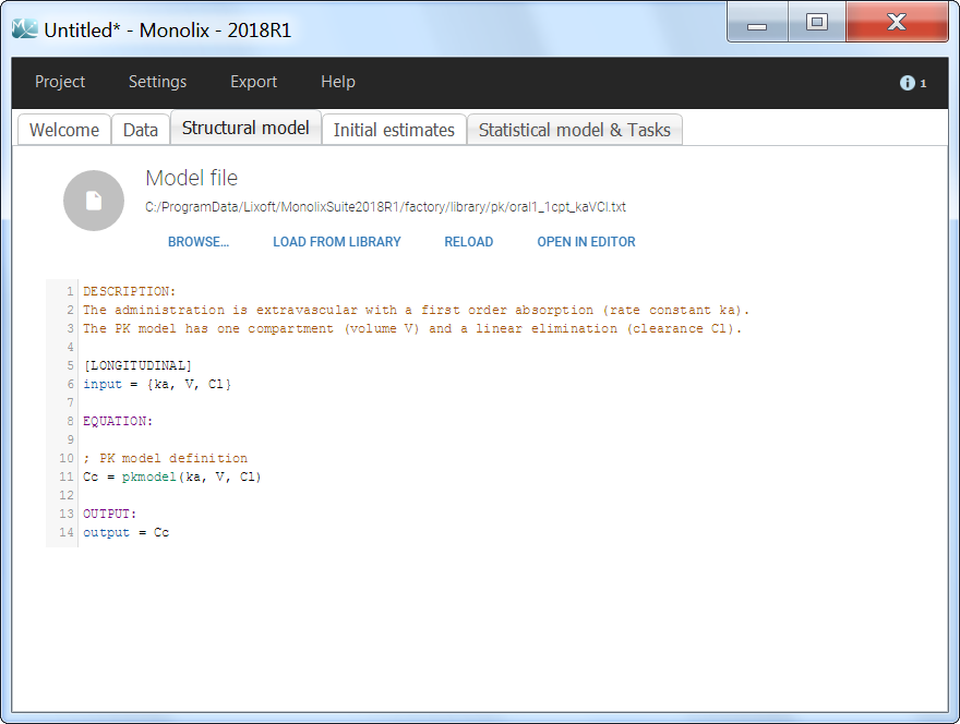
We would like to set up a one compartment PK model with first order absorption and linear elimination for the theophylline data set. We start by creating a new Monolix project. Next, the Data tab, click browse, and select the theophylline data set (which can be downloaded from the data set documentation webpage). In this example, all columns are already automatically tagged, based on the header names. We click ACCEPT and NEXT and arrive on the Structural model tab, click on LOAD FROM LIBRARY to choose a model from the Monolix libraries. The menu at the top allow to filter the list of models: after selecting an oral/extravascular administration, no delay, first-order absorption, one compartment and a linear elimination, two models remain in the list (ka,V,Cl) and (ka,V,k). Click on the oral1_1cpt_kaVCl.txt file to select it.
After this step, the GUI moves to the Initial Estimates tab, but it is possible to go back to the Structural model tab to see the content of the file:
[LONGITUDINAL]
input = {ka, V, Cl}

EQUATION:
Cc = pkmodel(ka, V, Cl)

OUTPUT:
output = Cc
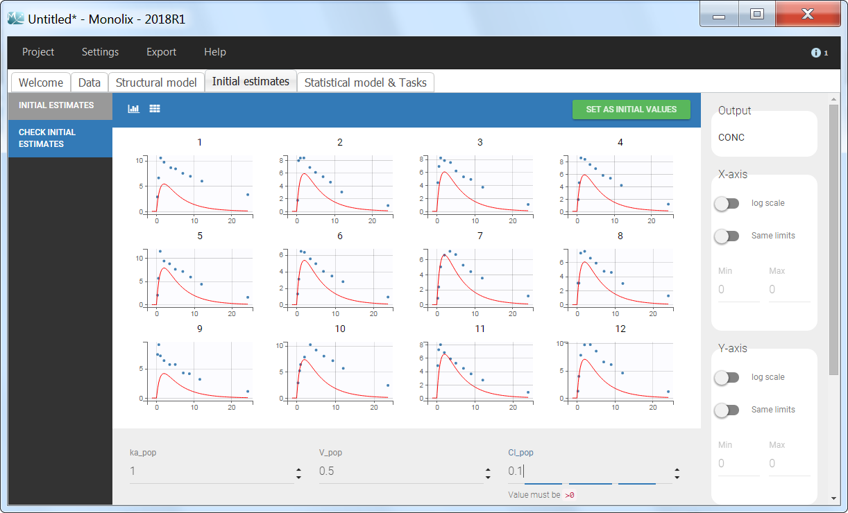
Back to the Initial Estimates tab, the initial values of the population parameters can be adjusted by comparing the model prediction using the chosen population parameters and the individual data. Click on SET AS INITIAL VALUES when you are done.
In the next tab, the Statistical model & Tasks tab, we propose by default:
- A combined error observation model
- Lognormal distributions for all parameters (ka, V and Cl)
At this stage, the monolix project should be saved. This creates a human readable text file with extension .mlxtran, which contains all the information defined via the GUI. In particular, the name of the model appears in the section [LONGITUDINAL] of the saved project file:
<MODEL>
[INDIVIDUAL]
input = {ka_pop, omega_ka, V_pop, omega_V, Cl_pop, omega_Cl}

DEFINITION:
ka = {distribution=lognormal, typical=ka_pop, sd=omega_ka}
V = {distribution=lognormal, typical=V_pop, sd=omega_V}
Cl = {distribution=lognormal, typical=Cl_pop, sd=omega_Cl}

[LONGITUDINAL]
input = {a, b}
file = 'lib:oral1_1cpt_kaVCl.txt'

DEFINITION:
CONC = {distribution=normal, prediction=Cc, errorModel=combined1(a,b)}
3.2.Writing your own model
If the models present in the libraries do not suit your needs, you can write a model yourself. You can either start completely from scratch or adapt a model existing in the libraries. In both cases, the syntax of the Mlxtran language is detailed on the mlxtran webpage. You can also copy-paste models from the mlxtran model example page.
Videos on this page use the application mlxEditor included in previous versions of MonolixSuite. From the 2021R1 version on, the editor is integrated within the interface of Monolix, as shown on the screenshots on this page, and it can also be used as a separate application.
Writing a model from scratch
- 8.case_studies/hcv_project (data = ‘hcv_data.txt’ , model=’hcvNeumann98_model.txt’)
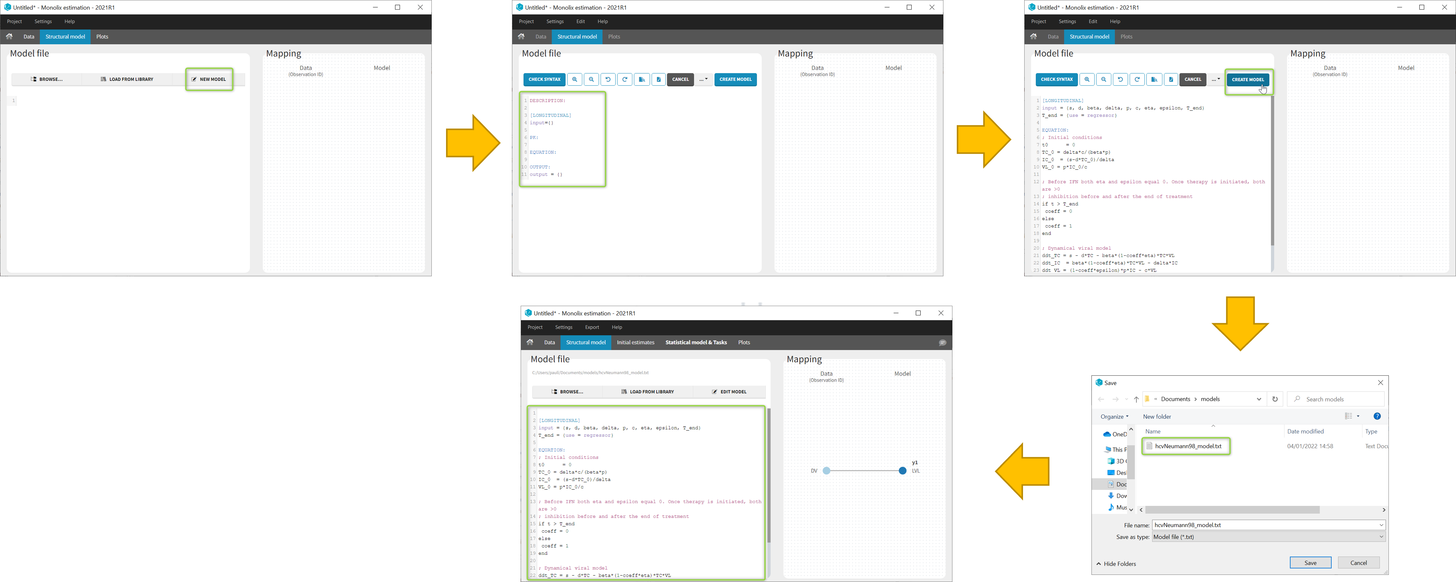
In the Structural model tab, you can click on New model to open the editor integrated within Monolix, and start writing your own model. The new model contains a convenient template defining the main blocks, input parameters and output variables. When you are done, click on Create model button of Monolix to save your new model file. After saving, the model is automatically loaded in the project.
You can even create your own library of models. An example of a basic library which includes several viral kinetics model is available in the demos 8.case_studies/model.
Note: A button “Check syntax” is available to check that there is no syntax error in the model. In case of an error, informative messages are displayed to help correct the error. The syntax check is also automatically applied before saving the model so that only a model with a valid syntax can be saved.
![]()
Understanding the error messages
The error messages generated when syntax errors are present in the model are very informative and quickly help to get the model right. The most common error messages are explained in detail in this video.
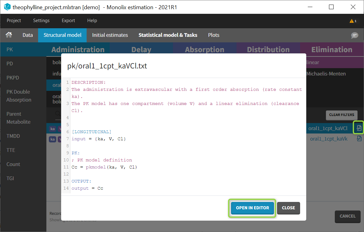
Modifying a model from the libraries
Browse existing models from the libraries using the Load from library button, then click the “file” icon next to a model name. This opens a pop-up window where the content of the model file is displayed. Click on Open in editor to open the model file in the MlxEditor. There you can adapt the model, for instance to add a PD model. Be careful to save the new model under a new name, to avoid overwriting the library files.
The video below shows an example of how a scale factor can be added:
See the dedicated webpage for more details on model libraries.
3.3.Models for continuous outcomes
3.3.1.Typical PK models
3.3.1.1.Single route of administration
- Introduction
- Intravenous bolus injection
- Intravenous infusion
- Oral administration
- Using different parametrizations
Objectives: learn how to define and use a PK model for single route of administration.
Projects: bolusLinear_project, bolusMM_project, bolusMixed_project, infusion_project, oral1_project, oral0_project, sequentialOral0Oral1_project, simultaneousOral0Oral1_project, oralAlpha_project, oralTransitComp_project
Introduction
Once a drug is administered, we usually describe subsequent processes within the organism by the pharmacokinetics (PK) process known as ADME: absorption, distribution, metabolism, excretion. A PK model is a dynamical system mathematically represented by a system of ordinary differential equations (ODEs) which describes transfers between compartments and elimination from the central compartment.
Mlxtran is remarkably efficient for implementing simple and complex PK models:
- The function
pkmodelcan be used for standard PK models. The model is defined according to the provided set of named arguments. Thepkmodelfunction enables different parametrizations, different models of absorption, distribution and elimination, defined here and summarized in the following.. - PK macros define the different components of a compartmental model. Combining such PK components provide a high degree of flexibility for complex PK models. They can also extend a custom ODE system.
- A system of ordinary differential equations (ODEs) can be implemented very easily.
It is also important to highlight the fact that the data file used by Monolix for PK modelling only contains information about dosing, i.e. how and when the drug is administrated. There is no need to integrate in the data file any information related to the PK model. This is an important remark since it means that any (complex) PK model can be used with the same data file. In particular, we make a clear distinction between administration (related to the data) and absorption (related to the model).
The pkmodel function
The PK model is defined by the names of the input parameters of the pkmodel function. These names are reserved keywords.
Absorption
- p: Fraction of dose which is absorbed
- ka: absorption constant rate (first order absorption)
- or, Tk0: absorption duration (zero order absorption)
- Tlag: lag time before absorption
- or, Mtt, Ktr: mean transit time & transit rate constant
Distribution
- V: Volume of distribution of the central compartment
- k12, k21: Transfer rate constants between compartments 1 (central) & 2 (peripheral)
- or V2, Q2: Volume of compartment 2 (peripheral) & inter compartment clearance, between compartments 1 and 2,
- k13, k31: Transfer rate constants between compartments 1 (central) & 3 (peripheral)
- or V3, Q3: Volume of compartment 3 (peripheral) & inter compartment clearance, between compartments 1 and 3.
Elimination
- k: Elimination rate constant
- or Cl: Clearance
- Vm, Km: Michaelis Menten elimination parameters
Effect compartment
- ke0: Effect compartment transfer rate constant
Intravenous bolus injection
Linear elimination
- bolusLinear_project
A single iv bolus is administered at time 0 to each patient. The data file bolus1_data.txt contains 4 columns: id, time, amt (the amount of drug in mg) and y (the measured concentration). The names of these columns are recognized as keywords by Monolix:
It is important to note that, in this data file, a row contains either some information about the dose (in which case y = ".") or a measurement (in which case amt = "."). We could equivalently use the data file bolus2_data.txt which contains 2 additional columns: EVID (in the green frame) and IGNORED OBSERVATION (in the blue frame):
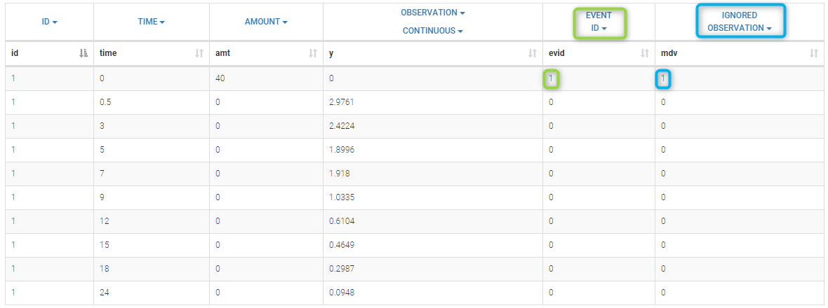 Here, the EVENT ID column allows the identification of an event. It is an integer between 0 and 4. It helps to define the type of line. EVID=1 means that this record describes a dose while EVID=0 means that this record contains an observed value.
On the other hand, the IGNORED OBSERVATION column enables to tag lines for which the information in the OBSERVATION column-type is missing. MDV=1 means that the observed value of this record should be ignored while MDV=0 means that this record contains an observed value. The two data files bolus1_data.txt and bolus2_data.txt contain exactly the same information and provide exactly the same results. A one compartment model with linear elimination is used with this project:
$$\begin{array}{ccl} \frac{dA_c}{dt} &=& – k A_c(t) \\ A_c(t) &= &0 ~~\text{for}~~ t<0 \end{array} $$
Here, \(A_c(t)\) and \(C_c(t)=A_c(t)/V\) are, respectively, the amount and the concentration of drug in the central compartment at time t. When a dose D arrives in the central compartment at time \(\tau\), an iv bolus administration assumes that
$$A_c(\tau^+) = A_c(\tau^-) + D$$
where \(A_c(\tau^-)\) (resp. \(A_c(\tau^+)\)) is the amount of drug in the central compartment just before (resp. after) \(\tau\) Parameters of this model are V and k. We therefore use the model bolus_1cpt_Vk from the Monolix PK library:
[LONGITUDINAL]
input = {V, k}

EQUATION:
Cc = pkmodel(V, k)

OUTPUT:
output = Cc
We could equivalently use the model bolusLinearMacro.txt (click on the button Model and select the new PK model in the library 6.PK_models/model)
[LONGITUDINAL]
input = {V, k}

PK:
compartment(cmt=1, amount=Ac)
iv(cmt=1)
elimination(cmt=1, k)
Cc = Ac/V

OUTPUT:
output = Cc
These two implementations generate exactly the same C++ code and then provide exactly the same results. Here, the ODE system is linear and Monolix uses its analytical solution. Of course, it is also possible (but not recommended with this model) to use the ODE based PK model bolusLinearODE.txt :
[LONGITUDINAL]
input = {V, k}

PK:
depot(target = Ac)

EQUATION:
ddt_Ac = - k*Ac
Cc = Ac/V

OUTPUT:
output = Cc
Results obtained with this model are slightly different from the ones obtained with the previous implementations since a numeric scheme is used here for solving the ODE. Moreover, the computation time is longer (between 3 and 4 time longer in that case) when using the ODE compared to the analytical solution.
Individual fits obtained with this model look nice
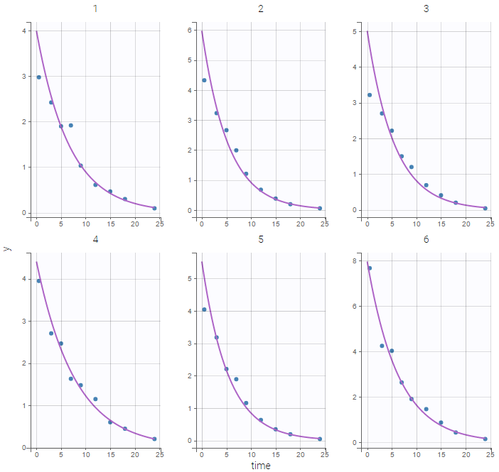
but the VPC show some misspecification in the elimination process:
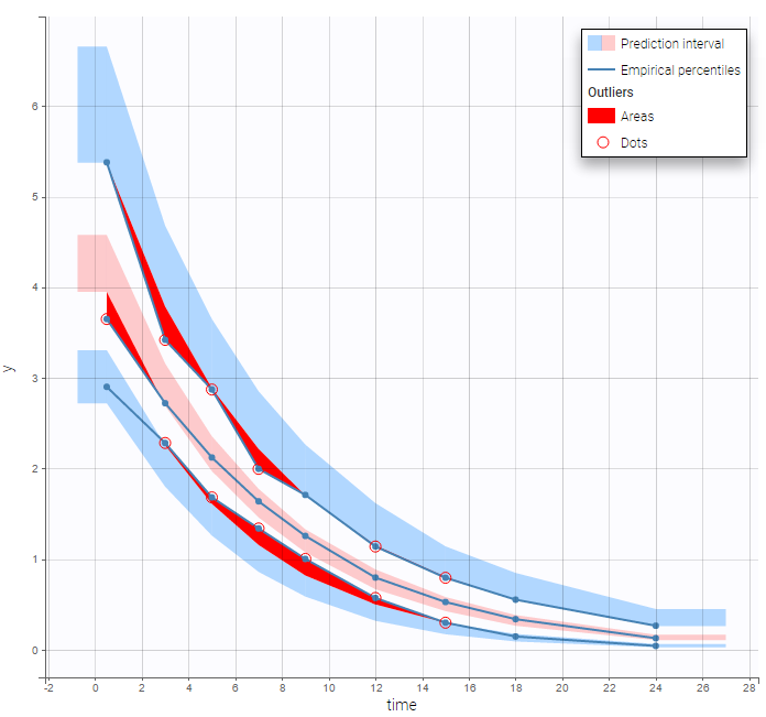
Michaelis Menten elimination
- bolusMM_project
A non linear elimination is used with this project:
$$\frac{dA_c}{dt} = – \frac{ V_m \, A_c(t)}{V\, K_m + A_c(t) }$$
This model is available in the Monolix PK library as bolus_1cpt_VVmKm:
[LONGITUDINAL]
input = {V, Vm, Km}

PK:
Cc = pkmodel(V, Vm, Km)

OUTPUT:
output = Cc
Instead of this model, we could equivalently use PK macros with bolusNonLinearMacro.txt from the library 6.PK_models/model:
[LONGITUDINAL]
input = {V, Vm, Km}

PK:
compartment(cmt=1, amount=Ac, volume=V)
iv(cmt=1)
elimination(cmt=1, Vm, Km)
Cc = Ac/V

OUTPUT:
output = Cc
or an ODE with bolusNonLinearODE:
[LONGITUDINAL]
input = {V, Vm, Km}

PK:
depot(target = Ac)

EQUATION:
ddt_Ac = -Vm*Ac/(V*Km+Ac)
Cc=Ac/V

OUTPUT:
output = Cc
Results obtained with these three implementations are identical since no analytical solution is available for this non linear ODE. We can then check that this PK model seems to describe much better the elimination process of the data:
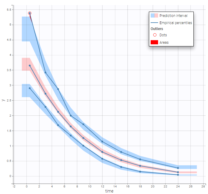
Mixed elimination
- bolusMixed_project
THe Monolix PK library contains “standard” PK models. More complex models should be implemented by the user in a model file. For instance, we assume in this project that the elimination process is a combination of linear and nonlinear elimination processes:
$$ \frac{dA_c}{dt} = -\frac{ V_m A_c(t)}{V K_m + A_c(t) } – k A_c(t) $$
This model is not available in the Monolix PK library. It is implemented in bolusMixed.txt:
[LONGITUDINAL]
input = {V, k, Vm, Km}

PK:
depot(target = Ac)

EQUATION:
ddt_Ac = -Vm*Ac/(V*Km+Ac) - k*Ac
Cc=Ac/V

OUTPUT:
output = Cc
This model, with a combined error model, seems to describe very well the data:
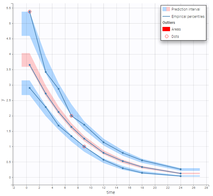
Intravenous infusion
- infusion_project
Intravenous infusion assumes that the drug is administrated intravenously with a constant rate (infusion rate), during a given time (infusion time). Since the amount is the product of infusion rate and infusion time, an additional column INFUSION RATE or INFUSION DURATION is required in the data file: Monolix can use both indifferently. Data file infusion_rate_data.txt has an additional column rate:
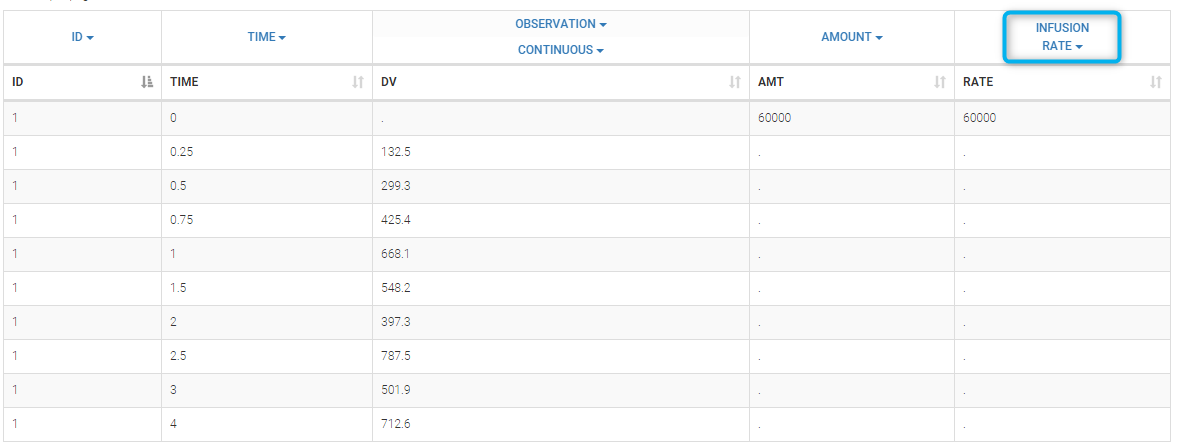
It can be replaced by infusion_tinf_data.txt which contains exactly the same information:
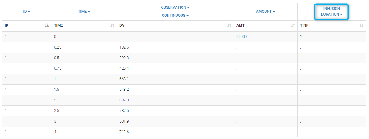
We use with this project a 2 compartment model with non linear elimination and parameters 


$$\begin{aligned} k_{12} &= Q/V_1 \\ k_{21} &= Q/V_2 \\\frac{dA_c}{dt} & = k_{21} \, Ap(t) – k_{12} \, Ac(t)- \frac{ V_m \, A_c(t)}{V_1\, K_m + A_c(t) } \\ \frac{dA_p}{dt} & = – k_{21} \, Ap(t) + k_{12} \, Ac(t) \\ Cc(t) &= \frac{Ac(t)}{V_1} \end{aligned}$$
This model is available in the Monolix PK library as infusion_2cpt_V1QV2VmKm:
[LONGITUDINAL]
input = {V1, Q, V2, Vm, Km}

PK:
V = V1
k12 = Q/V1
k21 = Q/V2
Cc = pkmodel(V, k12, k21, Vm, Km)

OUTPUT:
output = Cc
Oral administration
first-order absorption
- oral1_project
This project uses the data file oral_data.txt. For each patient, information about dosing is the time of administration and the amount. A one compartment model with first order absorption and linear elimination is used with this project. Parameters of the model are ka, V and Cl. we will then use model oral1_kaVCl.txt from the Monolix PK library
[LONGITUDINAL]
input = {ka, V, Cl}

EQUATION:
Cc = pkmodel(ka, V, Cl)

OUTPUT:
output = Cc
Both the individual fits and the VPCs show that this model doesn’t describe the absorption process properly.
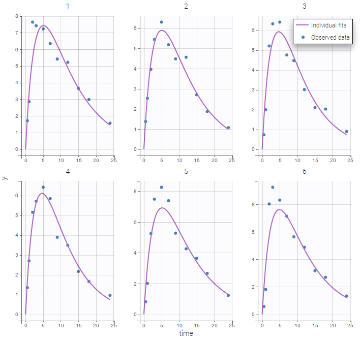
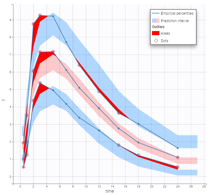 Many options for implementing this PK model with
 Mlxtran exists:
– using PK macros: oralMacro.txt:
[LONGITUDINAL]
input = {ka, V, Cl}

PK:
compartment(cmt=1, amount=Ac)
oral(cmt=1, ka)
elimination(cmt=1, k=Cl/V)
Cc=Ac/V

OUTPUT:
output = Cc
– using a system of two ODEs as in oralODEb.txt:
[LONGITUDINAL]
input = {ka, V, Cl}

PK:
depot(target=Ad)

EQUATION:
k = Cl/V
ddt_Ad = -ka*Ad
ddt_Ac =  ka*Ad - k*Ac
Cc = Ac/V

OUTPUT:
output = Cc
– combining PK macros and ODE as in oralMacroODE.txt (macros are used for the absorption and ODE for the elimination):
[LONGITUDINAL]
input = {ka, V, Cl}

PK:
compartment(cmt=1, amount=Ac)
oral(cmt=1, ka)

EQUATION:
k = Cl/V
ddt_Ac = - k*Ac
Cc = Ac/V

OUTPUT:
output = Cc
– or equivalently, as in oralODEa.txt:
[LONGITUDINAL]
input = {ka, V, Cl}

PK:
depot(target=Ac, ka)

EQUATION:
k = Cl/V
ddt_Ac = - k*Ac
Cc = Ac/V<

OUTPUT:
output = Cc
Remark: Models using the pkmodel function or PK macros only use an analytical solution of the ODE system.
zero-order absorption
- oral0_project
A one compartment model with zero order absorption and linear elimination is used to fit the same PK data with this project. Parameters of the model are Tk0, V and Cl. We will then use model oral0_1cpt_Tk0Vk.txt from the Monolix PK library
[LONGITUDINAL]
input = {Tk0, V, Cl}

EQUATION:
Cc = pkmodel(Tk0, V, Cl)

OUTPUT:
output = Cc
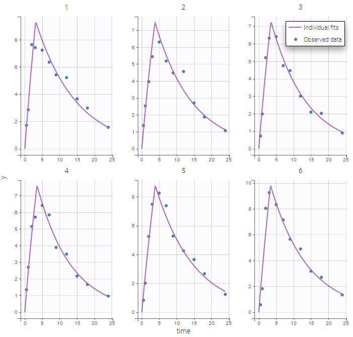
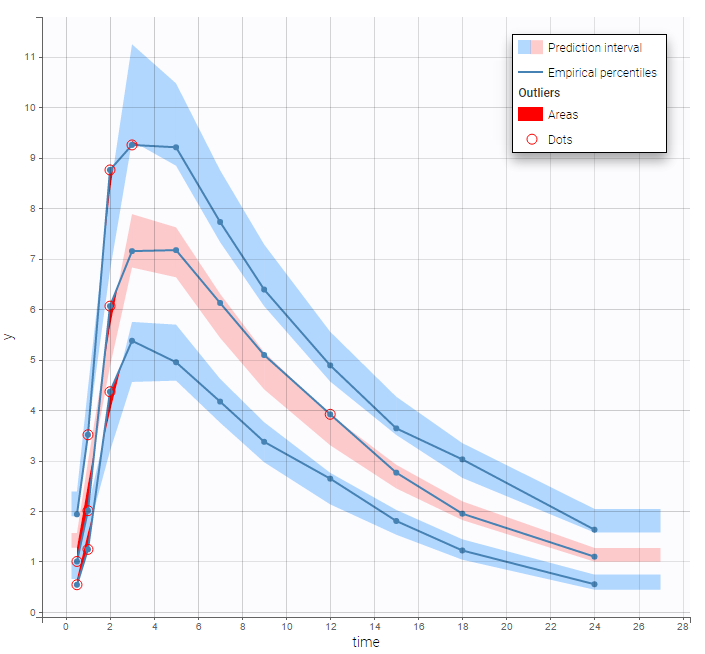
Remark 1: implementing a zero-order absorption process using ODEs is not easy… on the other hand, it becomes extremely easy to implement using either the pkmodel function or the PK macro oral(Tk0).
Remark 2: The duration of a zero-order absorption has nothing to do with an infusion time: it is a parameter of the PK model (exactly as the absorption rate constant ka for instance), it is not part of the data.
sequential zero-order first-order absorption
- sequentialOral0Oral1_project
More complex PK models can be implemented using Mlxtran. A sequential zero-order first-order absorption process assumes that a fraction Fr of the dose is first absorbed during a time Tk0 with a zero-order process, then, the remaining fraction is absorbed with a first-order process. This model is implemented in sequentialOral0Oral1.txt using PK macros:
[LONGITUDINAL]
input = {Fr, Tk0, ka, V, Cl}

PK:
compartment(amount=Ac)
absorption(Tk0, p=Fr)
absorption(ka, Tlag=Tk0, p=1-Fr)
elimination(k=Cl/V)
Cc=Ac/V

OUTPUT:
output = Cc
Both the individual fits and the VPCs show that this PK model describes very well the whole ADME process for the same PK data:
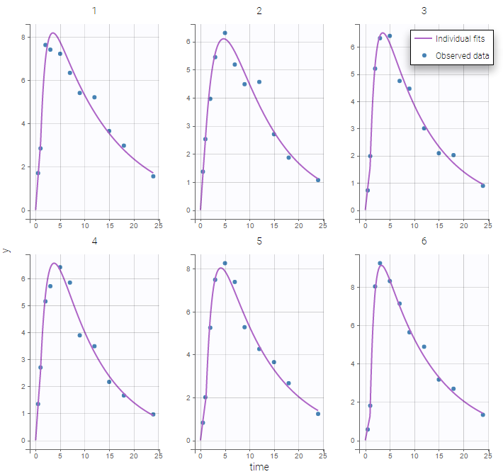
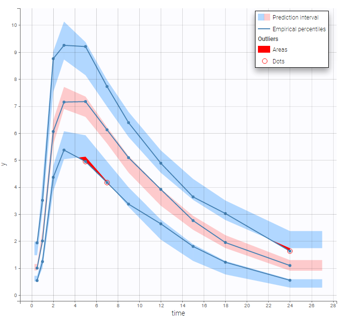
simultaneous zero-order first-order absorption
- simultaneousOral0Oral1_project
A simultaneous zero-order first-order absorption process assumes that a fraction Fr of the dose is absorbed with a zero-order process while the remaining fraction is absorbed simultaneously with a first-order process. This model is implemented in simultaneousOral0Oral1.txt using PK macros:
[LONGITUDINAL]
input = {Fr, Tk0, ka, V, Cl}

PK:
compartment(amount=Ac)
absorption(Tk0, p=Fr)
absorption(ka, p=1-Fr)
elimination(k=Cl/V)
Cc=Ac/V

OUTPUT:
output = Cc
alpha-order absorption
- oralAlpha_project
An 
\right)^\alpha")
This model is implemented in oralAlpha.txt using ODEs:
[LONGITUDINAL]
input = {r, alpha, V, Cl}

PK:
depot(target = Ad)

EQUATION:
dAd = Ad^alpha
ddt_Ad = -r*dAd
ddt_Ac = r*Ad - (Cl/V)*Ac
Cc = Ac/V

OUTPUT:
output = Cc
transit compartment model
- oralTransitComp_project
A PK model with a transit compartment of transit rate Ktr and mean transit time Mtt can be implemented using the PK macro oral(ka, Mtt, Ktr), or using the pkmodel function, as in oralTransitComp.txt:
[LONGITUDINAL]
input = {Mtt, Ktr, ka, V, Cl}

EQUATION:
Cc = pkmodel(Mtt, Ktr, ka, V, Cl)

OUTPUT:
output = Cc
Using different parametrizations
The PK macros and the function pkmodel use some preferred parametrizations and some reserved names as input arguments: Tlag, ka, Tk0, V, Cl, k12, k21. It is however possible to use another parametrization and/or other parameter names. As an example, consider a 2-compartment model for oral administration with a lag, a first order absorption and a linear elimination. We can use the pkmodel function with, for instance, parameters ka, V, k, k12 and k21:
[LONGITUDINAL]
input = {ka, V, k, k12, k21}

PK:
Cc = pkmodel(ka, V, k, k12, k21)

OUTPUT:
output = Cc
Imagine now that we want i) to use the clearance 

[LONGITUDINAL]
input = {KA, V, CL, K12, K21}

PK:
Cc = pkmodel(ka=KA, V, k=CL/V, k12=K12, k21=K21)

OUTPUT:
output = Cc
3.3.1.2.Multiple routes of administration
Objectives: learn how to define and use a PK model for multiple routes of administration..
Projects: ivOral1_project, ivOral2_project
Some drugs can display complex absorption kinetics. Common examples are mixed first-order and zero-order absorptions, either sequentially or simultaneously, and fast and slow parallel first-order absorptions. A few examples of those kinds of absorption kinetics are proposed below. Various absorption models are proposed here as examples.
Combining iv and oral administrations – Example 1
- ivOral1_project (data = ‘ivOral1_data.txt’ , model = ‘ivOral1Macro_model.txt’)
In this example, we combine oral and iv administrations of the same drug. The data file ivOral1_data.txt contains an additional column ADMINISTRATION ID which indicates the route of administration (1=iv, 2=oral)
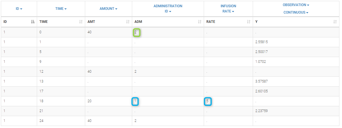
We assume here a one compartment model with first-order absorption process from the depot compartment (oral administration) and a linear elimination process from the central compartment. We further assume that only a fraction F (bioavailability) of the drug orally administered is absorbed. This model is implemented in ivOral1Macro_model.txt using PK macros:
[LONGITUDINAL]
input = {F, ka, V, k}

PK:
compartment(cmt=1, amount=Ac)
iv(adm=1, cmt=1)
oral(adm=2, cmt=1, ka, p=F)
elimination(cmt=1, k)
Cc = Ac/V

OUTPUT:
output = Cc
A logit-normal distribution is used for bioavability F that takes it values in (0,1). The model properly fits the data as can be seen on the individual fits of the 6 first individuals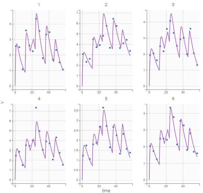
Remark: the same PK model could be implemented using ODEs instead of PK macros.
Let \(A_d\) and \(A_c\) be, respectively, the amounts in the depot compartment (gut) and the central compartment (bloodtsream). Kinetics of \(A_d\) and \(A_c\) are described by the following system of ODEs
$$\dot{A}_d(t) = – k_a A_d(t)~~\text{and}~~ \dot{A}_c(t) = k_a A_d(t) – k A_c(t)$$
The target compartment is the depot compartment (\(A_d\)) for oral administrations and the central compartment (\(A_c\)) for iv administrations. This model is implemented in ivOral1ODE_model.txt using a system of ODEs:
[LONGITUDINAL]
input = {F, ka, V, k}

PK:
depot(type=1, target=Ad, p=F)
depot(type=2, target=Ac)

EQUATION:
ddt_Ad = -ka*Ad
ddt_Ac =  ka*Ad - k*Ac
Cc = Ac/V

OUTPUT:
output = Cc
Solving this ODEs system is less efficient than using the PK macros which uses the analytical solution of the linear system.
Combining iv and oral administrations – Example 2
- ivOral2_project (data = ‘ivOral2_data.txt’ , model = ‘ivOral2Macro_model.txt’)
In this example (based on simulated PK data), we combine intraveinous injection with 3 different types of oral administrations of the same drug. The datafile ivOral2_data.txt contains column ADM which indicates the route of administration (1,2,3=oral, 4=iv). We assume that one type of oral dose (adm=1) is absorbed into a latent compartment following a zero-order absorption process. The 2 oral doses (adm=2,3) are absorbed into the central compartment following first-order absorption processes with different rates. Bioavailabilities are supposed to be different for the 3 oral doses. There is linear transfer from the latent to the central compartment. A peripheral compartment is linked to the central compartment. The drug is eliminated by a linear process from the central compartment:
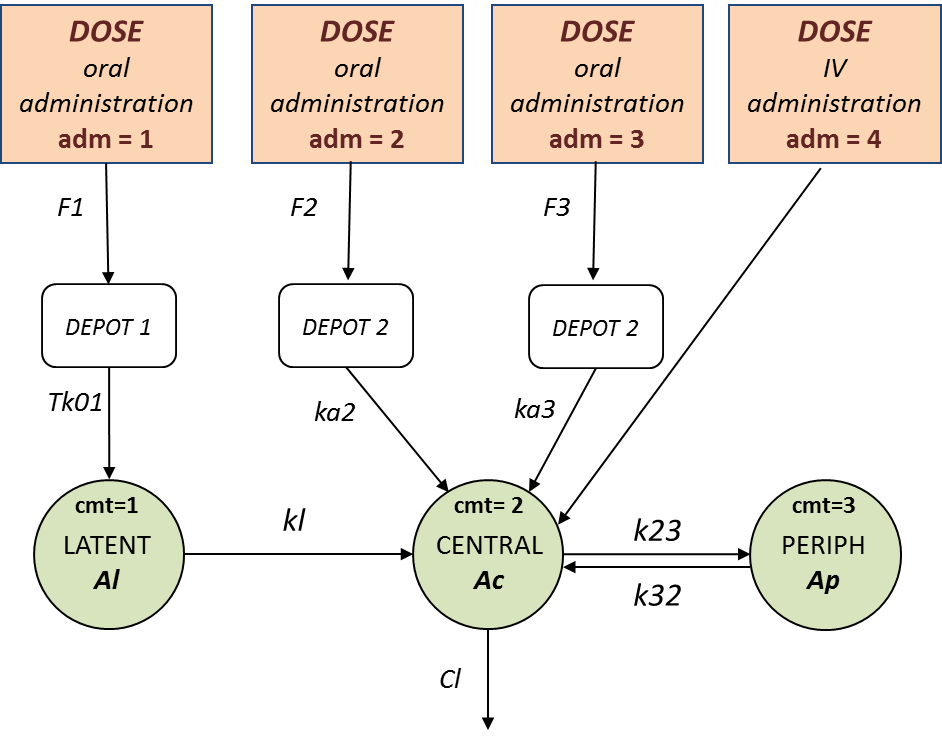
This model is implemented in ivOral2Macro_model.txt using PK macros:
[LONGITUDINAL]
input = {F1, F2, F3, Tk01, ka2, ka3, kl, k23, k32, V, Cl}

PK:
compartment(cmt=1, amount=Al)
compartment(cmt=2, amount=Ac)
peripheral(k23,k32)
oral(type=1, cmt=1, Tk0=Tk01, p=F1)
oral(type=2, cmt=2, ka=ka2,   p=F2)
oral(type=3, cmt=2, ka=ka3,   p=F3)
iv(type=4, cmt=2)
transfer(from=1, to=2, kt=kl)
elimination(cmt=2, k=Cl/V)
Cc = Ac/V

OUTPUT:
output = Cc
Here, logit-normal distributions are used for bioavabilities \(F_1\), \(F_2\) and \(F_3\). The model fits the data properly :
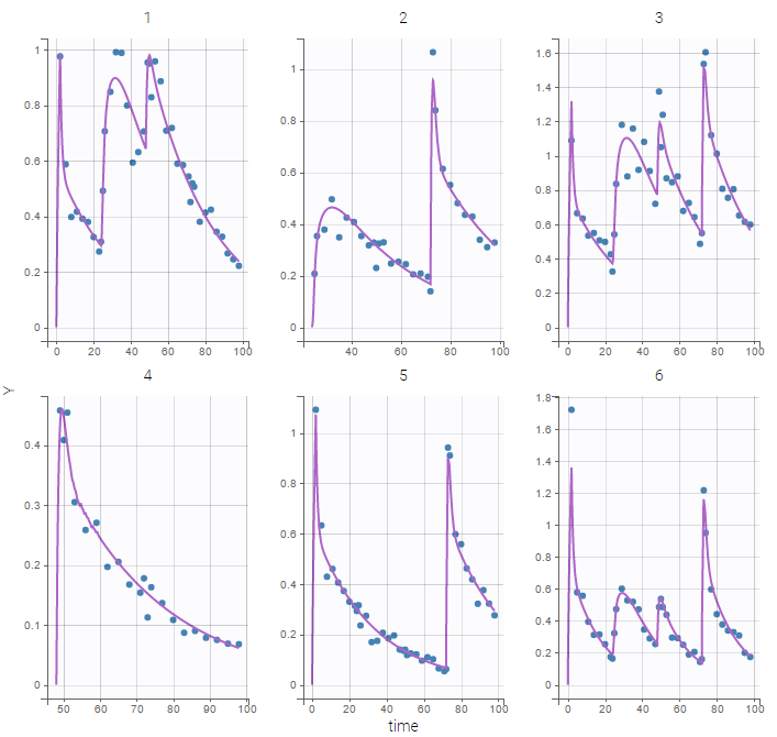
Remark: the number and type of doses vary from one patient to another in this example.
3.3.1.3.Multiple doses to steady-state
Objectives: learn how to define and use a PK model with multiple doses or assuming steady-state.
Projects: multidose_project, addl_project, ss1_project, ss2_project, ss3_project
Multiple doses
- multidose_project (data = ‘multidose_data.txt’ , model = ‘lib:bolus_1cpt_Vk.txt’)
In this project, each patient receives several iv bolus injections. Each dose is represented by a row in the data file multidose_data.txt:
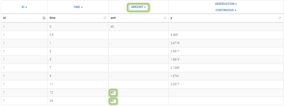
The PK model and the statistical model used in this project properly fit the observed data of each individual. Even if there is no observation between 12h and 72h, predicted concentrations computed on this time interval exhibit the multiple doses received by each patient:
VPCs, which is a diagnosis tool, are based on the design of the observations and therefore “ignore” what may happen between 12h and 72h:
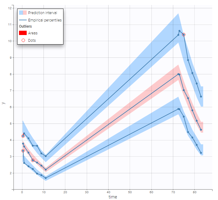
On the other hand, the prediction distribution, which is not a diagnosis tool, computes the distribution of the predicted concentration at any time point:
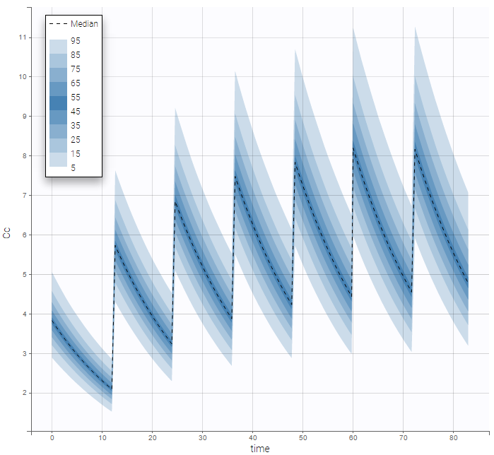
Additional doses (ADDL)
- addl_project (data = ‘addl_data.txt’ , model = ‘lib:bolus_1cpt_Vk.txt’)
We can note in the previous project, that, for each patient, the interval time between two successive doses is the same (12 hours for each patient) and the amount of drug which is administrated is always the same as well (40mg for each patient). We can take advantage of this design in order to simplify the data file by defining, for each patient, a unique amount (AMT), the number of additional doses which are administrated after the first one (ADDITIONAL DOSES) and the time interval between successive doses (INTERDOSE INTERVAL):
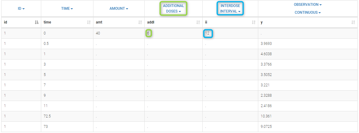
The keywords ADDL and II are automatically recognized by Monolix.
Remarks:
- Results obtained with this project, i.e. with this data file, are identical to the ones obtained with the previous project.
- It is possible to combine single doses (using ADDL=0) and repeated doses in a same data file.
Steady-state
- ss1_project (data = ‘ss1_data.txt’ , model = ‘lib:oral0_1cpt_Tk0VCl.txt’)
The dose, orally administrated at time 0 to each patient, is assumed to be a “steady-state dose” which means that a “large” number of doses before time 0 have been administrated, with a constant amount and a constant interval dosing, such that steady-state, i.e. equilibrium, is reached at time 0. The data file ss1_data contains a column STEADY STATE which indicates if the dose is a steady-state dose or not and a column INTERDOSE INTERVAL for the inter-dose interval:

Click on Check the initial fixed effects to display the predicted concentration between the last dose administrated at time 0. One can see that the initial concentration is not 0 but the result of the steady state calculation.
 We see on this plot that Monolix adds 5 doses before the last dose to reach steady-state. Individual fits display the predicted concentrations computed with these additional doses:

If the dynamics is slow, adding 5 doses before the last dose might not be sufficient. You can adapt the number of doses in the frame data and thus define it for all individuals as on the following figure.

leading to the following check initial fixed effects
- ss2_project (data = ‘ss2_data.txt’ , model = ‘lib:oral0_1cpt_Tk0VCl.txt’)
Steady-state and non steady-sates doses are combined in this project:

Individual fits display the predicted concentrations computed with this combination of doses:

3.3.2.Mixture of structural models
- Introduction
- Between subject mixture models
- Supervised learning (with regressor)
- Unsupervised learning (with bsmm function)
- Within subject mixture models
Objectives: learn how to implement between subject mixture models (BSMM) and within subject mixture models (WSMM).
Projects: bsmm1_project, bsmm2_project, wsmm_project
Introduction
There are two approaches to define a mixture of models:
- defining a mixture of structural models (via a regressor or via the bsmm function). This approach is detailed here.
- introducing a categorical covariate (known or latent). –> click here to go to the page dedicated to this approach.
Several types of mixture models exist, they are useful in the context of mixed effects models. It may be necessary in some situations to introduce diversity into the structural models themselves:
- Between-subject model mixtures (BSMM) assume that there exists subpopulations of individuals. Different structural models describe the response of each subpopulation, and each subject belongs to one of these subpopulations. One can imagine for example different structural models for responders, nonresponders and partial responders to a given treatment.
The easiest way to model a finite mixture model is to introduce a label sequence ")


")
$$f\left(t_{ij}; \psi_i, z_i \right) = \sum_{m=1}^M 1_{z_i = m} f_m\left( t_{ij}; \psi_i \right) $$
In other word, each subpopulation has its own structural model: 
- Within-subject model mixtures (WSMM) assume that there exist subpopulations (of cells, viruses, etc.) within each patient. In this case, different structural models can be used to describe the response of different subpopulations, but the proportion of each subpopulation depends on the patient.
Then, it makes sense to consider that the mixture of models happens within each individual. Such within-subject model mixtures require additional vectors of individual parameters ")
$$f\left( t_{ij}; \psi_i, z_i \right) = \sum_{m=1}^M \pi_{m,i} f_m\left( t_{ij}; \psi_i \right)$$
The proportions ")
Between subject mixture models
Supervised learning
- bsmm1_project (data = ‘pdmixt1_data.txt’, model = ‘bsmm1_model.txt’)
We consider a very simple example here with two subpopulations of individuals who receive a given treatment. The outcome of interest is the measured effect of the treatment (a viral load for instance). The two populations are non responders and responders. We assume here that the status of the patient is known. Then, the data file contains an additional column GROUP. This column is duplicated because Monolix uses it
- i) as a regression variable (REGRESSOR): it is used in the model to distinguish responders and non responders,
- ii) as a categorical covariate (CATEGORICAL COVARIATE): it is used to stratify the diagnosis plots.
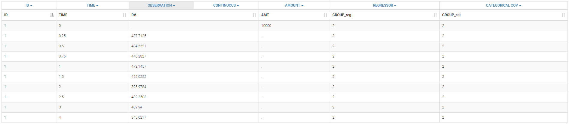
We can then display the data
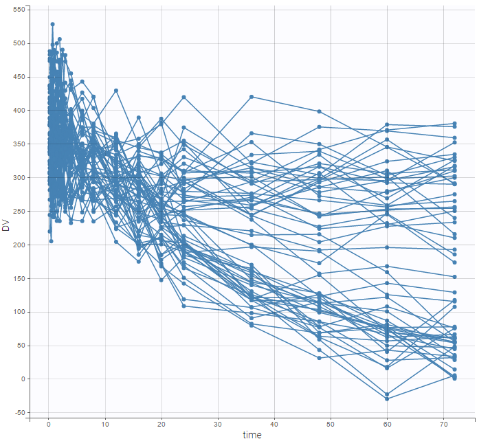
and use the categorical covariate GROUP_CAT to split the plot into responders and non responders:
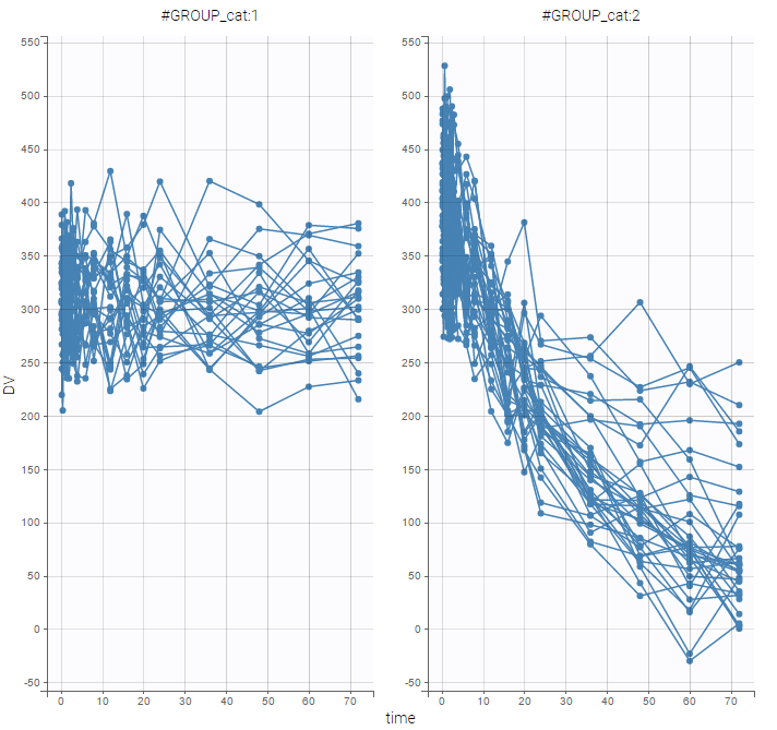 We use different structural models for non responders and responders. The predicted effect for non responders is constant f(t) = A1 while the predicted effect for responders decreases exponentially f(t) = A2 exp(-kt).
The model is implemented in the model file bsmm1_model.txt (note that the names of the regression variable in the data file and in the model script do not need to match):
[LONGITUDINAL]
input = {A1, A2, k, g}
g = {use=regressor}

EQUATION:
if g==1
   f = A1
else
   f = A2*exp(-k*max(t,0))
end

OUTPUT:
output = f
The plot of individual fits exhibit the two different structural models:
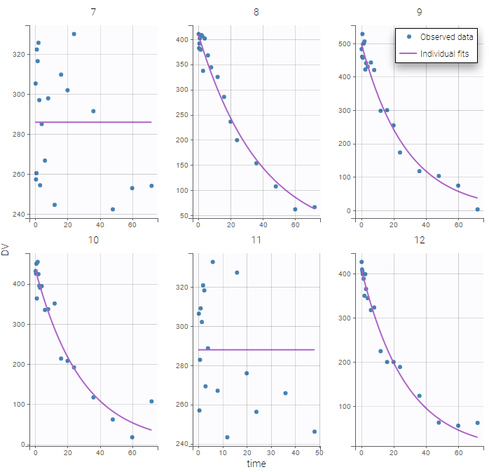
VPCs should then be splitted according to the GROUP_CAT
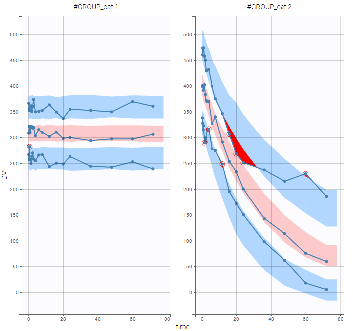
as well as the prediction distribution for non responders and responders:
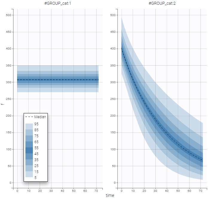
Unsupervised learning
- bsmm2_project (data = ‘pdmixt2_data.txt’, model = ‘bsmm2_model.txt’)
The status of the patient is unknown in this project (which means that the column GROUP is not available anymore). Let p be the proportion of non responders in the population. Then, the structural model for a given subject is f1 with probability p and f2 with probability 1-p. The structural model is therefore a BSMM:
[LONGITUDINAL]
input = {A1, A2, k, p}

EQUATION:
f1 = A1
f2 = A2*exp(-k*max(t,0))
f  = bsmm(f1, p, f2, 1-p)

OUTPUT:
output = f
Important:
- The bsmm function must be used on the last line of the structural model, just before “OUTPUT:”. It is not possible to reuse the variable returned by the bsmm function (here f) in another equation.
- p is a population parameter of the model to estimate. There is no inter-patient variability on p: all the subjects have the same probability of being a non responder in this example. We use a logit-normal distribution for p in order to constrain it to be between 0 and 1, but without variability:
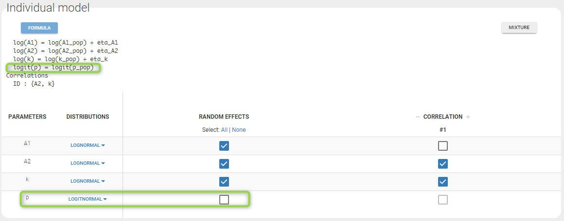 p is estimated with the other population parameters:
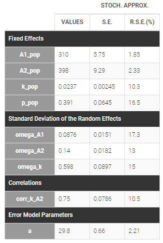
Then, the group to which a patient belongs is also estimated as the group of highest conditional probability:
$$\begin{aligned}\hat{z}_i &= 1~~~~\textrm{if}~~~~ \mathbb{P}(z_i=1 | (y_{ij}), \hat{\psi}_i, \hat{\theta})> \mathbb{P}(z_i=2 | (y_{ij}),\hat{\psi}_i, \hat{\theta}),\\ &=0~~~~\textrm{otherwise}\end{aligned}$$
The estimated groups can be used as a stratifying variable to split some plots such as VPCs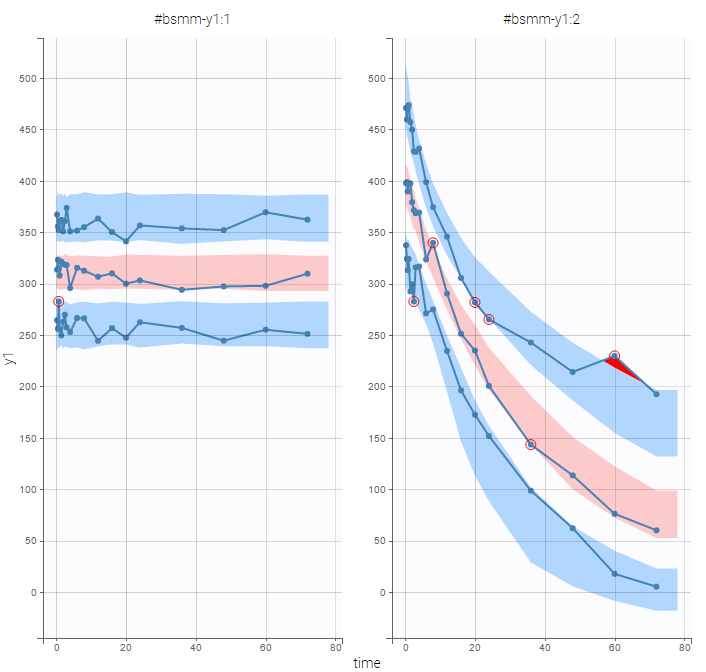
Bsmm function with ODEs
The bsmm function can also be used with models defined via ODE systems. The syntax in that case follows this example, with model M defined as a mixture of M1 and M2:
M1_0 = ... ; initial condition for M1
ddt_M1 = ... ; ODE for M1
M2_0 = ... ; initial condition for M2
ddt_M2 = ... ; ODE for M2

M = bsmm(M1,p1,M2,1-p1)
Unsupervised learning with latent covariates
If the models composing the mixture have a similar structure, it is sometimes possible and easier to implement the mixture with a latent categorical covariate instead of the bsmm function. It also has the advantage of allowing more than two mixture groups, while the bsmm function can only define two mixture groups.
Within subject mixture models
- wsmm_project (data = ‘pdmixt2_data.txt’, model = ‘wsmm_model.txt’)
It may be too simplistic to assume that each individual is represented by only one well-defined model from the mixture. We consider here that the mixture of models happens within each individual and use a WSMM: f = p*f1 + (1-p)*f2
[LONGITUDINAL]
input = {A1, A2, k, p}

EQUATION:
f1 = A1
f2 = A2*exp(-k*max(t,0))
f = wsmm(f1, p, f2, 1-p)

OUTPUT:
output = f
Remark: Here, writing f = wsmm(f1, p, f2, 1-p) is equivalent to writing f = p*f1 + (1-p)*f2
Important: Here, p is an individual parameter: the subjects have different proportions of non responder cells. We use a probit-normal distribution for p in order to constrain it to be between 0 and 1, with variability:
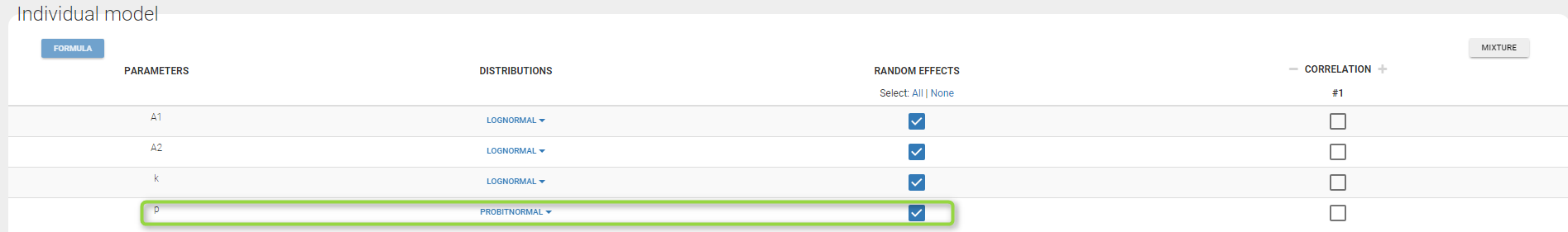
There is no latent covariate when using WSMM: mixtures are continuous mixtures. We therefore cannot split anymore the VPC and the prediction distribution anymore.
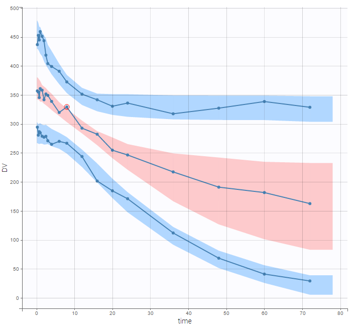 |
 |
|---|
3.3.3.Joint models for continuous outcomes
- Introduction
- Fitting first a PK model to the PK data
- Simultaneous PKPD modeling
- Sequential PKPD modelling
- Fitting a PKPD model to the PD data only
- Case studies
Objectives: learn how to implement a joint model for continuous PKPD data.
Projects: warfarinPK_project, warfarin_PKPDimmediate_project, warfarin_PKPDeffect_project, warfarin_PKPDturnover_project, warfarin_PKPDseq1_project, warfarin_PKPDseq2_project, warfarinPD_project
Introduction
A “joint model” describes two or more types of observation that typically depend on each other. A PKPD model is a “joint model” because the PD depends on the PK. Here we demonstrate how several observations can be modeled simultaneously. We also discuss the special case of sequential PK and PD modelling, using either the population PK parameters or the individual PK parameters as an input for the PD model.
Fitting first a PK model to the PK data
- warfarinPK_project (data = ‘warfarin_data.txt’, model = ‘lib:oral1_1cpt_TlagkaVCl.txt’)
The column DV of the data file contains both the PK and the PD measurements: in Monolix this column is tagged as an OBSERVATION column. The column DVID is a flag defining the type of observation: DVID=1 for PK data and DVID=2 for PD data: the keyword OBSERVATION ID is then used for this column.
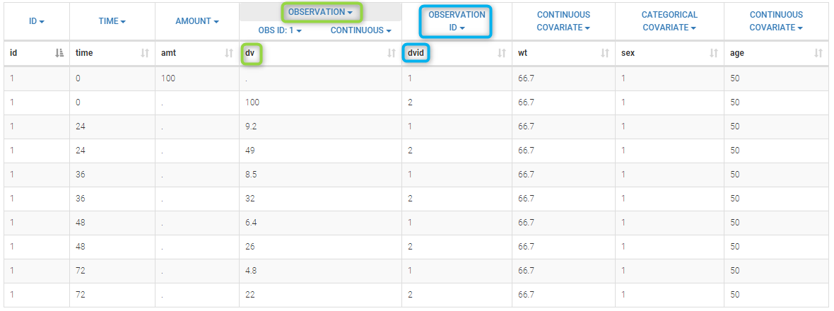 We will use the model oral1_1cpt_TlagkaVCl from the
 Monolix PK library
[LONGITUDINAL]
input = {Tlag, ka, V, Cl}

EQUATION:
Cc = pkmodel(Tlag, ka, V, Cl)

OUTPUT:
output = {Cc}
Only the predicted concentration Cc is defined as an output of this model. Then, this prediction will be automatically associated to the outcome of type 1 (DVID=1) while the other observations (DVID=2) will be ignored.
Remark: any other ordered values could be used for OBSERVATION ID column: the smallest one will always be associated to the first prediction defined in the model.
Simultaneous PKPD modeling
- warfarin_PKPDimmediate_project (data = ‘warfarin_data.txt’, model = ‘immediateResponse_model.txt’)
It is also possible for the user to write his own PKPD model. The same PK model used previously and an immediate response model are defined in the model file immediateResponse_model.txt
[LONGITUDINAL]
input = {Tlag, ka, V, Cl, Imax, IC50, S0}

EQUATION:
Cc = pkmodel(Tlag, ka, V, Cl)
E = S0 * (1 - Imax*Cc/(Cc+IC50))

OUTPUT:
output = {Cc, E}
Two predictions are now defined in the model: Cc for the PK (DVID=1) and E for the PD (DVID=2).
- warfarin_PKPDeffect_project (data = ‘warfarin_data.txt’, model = ‘effectCompartment_model.txt’)
An effect compartment is defined in the model file effectCompartment_model.txt
[LONGITUDINAL]
input = {Tlag, ka, V, Cl, ke0, Imax, IC50, S0}

EQUATION:
{Cc, Ce} = pkmodel(Tlag, ka, V, Cl, ke0)
E = S0 * (1 - Imax*Ce/(Ce+IC50))

OUTPUT:
output = {Cc, E}
Ce is the concentration in the effect compartment
- warfarin_PKPDturnover_project (data = ‘warfarin_data.txt’, model = ‘turnover1_model.txt’)
An indirect response (turnover) model is defined in the model file turnover1_model.txt
[LONGITUDINAL]
input =  {Tlag, ka, V, Cl, Imax, IC50, Rin, kout}

EQUATION:
Cc = pkmodel(Tlag, ka, V, Cl)
E_0 = Rin/kout
ddt_E = Rin*(1-Imax*Cc/(Cc+IC50)) - kout*E

OUTPUT:
output = {Cc, E}
Sequential PKPD modelling
In the sequential approach, a PK model is developed and parameters are estimated in the first step. For a given PD model, different strategies are then possible for the second step, i.e., for estimating the population PD parameters:
Using estimated population PK parameters
- warfarin_PKPDseq1_project (data = ‘warfarin_data.txt’, model = ‘turnover1_model.txt’)
Population PK parameters are set to their estimated values but individual PK parameters are not assumed to be known and sampled from their conditional distributions at each SAEM iteration. In Monolix, this simply means changing the status of the population PK parameter values so that they are no longer used as initial estimates for SAEM but considered fixed as on the figure below.

To fix parameters, click on the green option button (framed in green) and choose the Fixed method as on the figure below

The joint PKPD model defined in turnover1_model.txt is again used with this project.
Using estimated individual PK parameters
- warfarin_PKPDseq2_project (data = ‘warfarinSeq_data.txt’, model = ‘turnoverSeq_model.txt’)
In htis case, individual PK parameters are set to their estimated values and used as constants in the PKPD model to fit the PD data. To do so, the individual PK parameters need to be added to the PD dataset (or PK/PD dataset) and tagged as regressors.
The PK project (that was executed before and through which the estimated PK parameters were obtained) contains in the result folder the individual parameter values “..\warfarin_PKPDseq1_project\IndividualParameters\estimatedIndividualParameters.txt”. These estimated PK parameters can be added to the PD dataset by using the data formatting tool integrated in Monolix version 2023R1. Depending which tasks have been run in the PK project, the individual parameters corresponding to the conditional mode (EBEs, with “_mode”), the conditional mean (mean of the samples from the conditional distributions, with “_mean”) and an approximation of the conditional mean obtained at the end of the SAEM step (with “_SAEM”) are available in the file. All columns are added to the PD dataset.
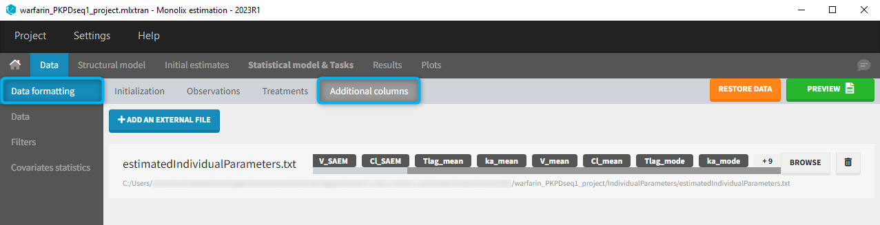
At the data tagging step, the user can choose which individual parameters to use. The most common is to use the EBEs so to tag the columns with “_mode” as regressor and leave the others as IGNORE (purple frame below). By activating the toggle button (green frame), the ignored columns flagged with the keyword IGNORE can be hidden.
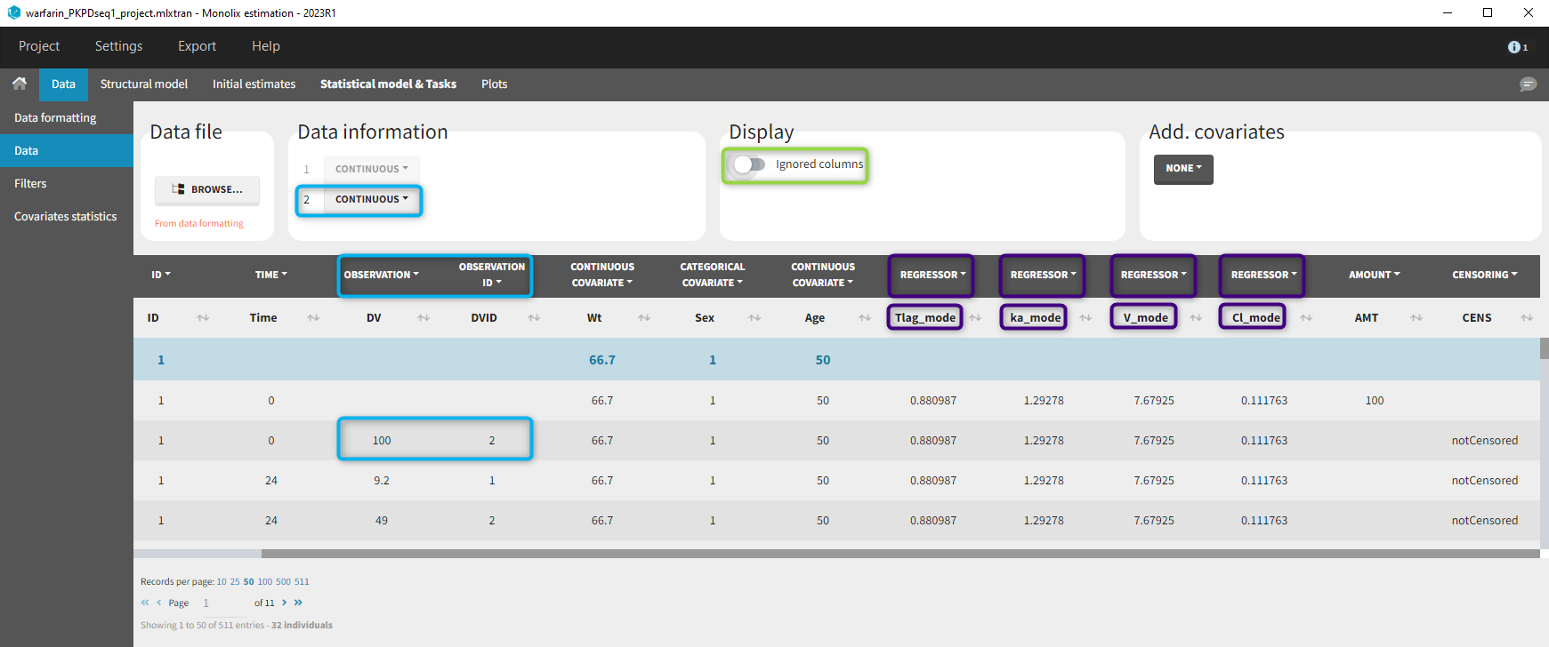
We use the same turnover model for the PD data. Here, the PK parameters are defined as regression variables (i.e. regressors).
[LONGITUDINAL]
input =  {Imax, IC50, Rin, kout, Tlag, ka, V, Cl}
Tlag  = {use = regressor}
ka    = {use = regressor}
V     = {use = regressor}
Cl    = {use = regressor}

EQUATION:
Cc = pkmodel(Tlag,ka,V,Cl)
E_0 = Rin/kout
ddt_E= Rin*(1-Imax*Cc/(Cc+IC50)) - kout*E

OUTPUT:
output = {E}
As you can see, the names of the regressors do not match the parameter names. The regressors are matched by order (not by name) between the data set and the model input statement.
If there are multiple observation types in the data as well as different response vectors in the output statement of the structural model, then these must be mapped accordingly in the mapping panel.
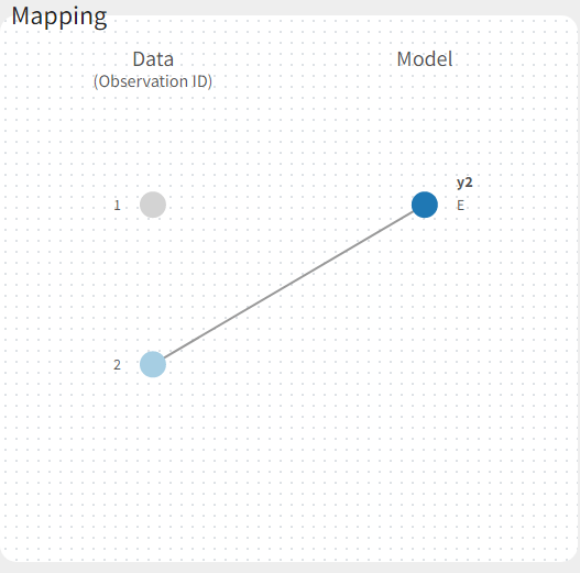
Fitting a PKPD model to the PD data only
- warfarinPD_project (data = ‘warfarinPD_data.txt’, model = ‘turnoverPD_model.txt’)
In this example, only PD data is available. Nevertheless, a PKPD model – where only the effect is defined as a prediction – can be used for fitting this data and thus defined in the OUTPUT section.
[LONGITUDINAL]
input =  {Tlag, ka, V, Cl, Imax, IC50, Rin, kout}

EQUATION:
Cc = pkmodel(Tlag, ka, V, Cl)
E_0 = Rin/kout
ddt_E = Rin*(1-Imax*Cc/(Cc+IC50)) - kout*E

OUTPUT:
output = {E}
Case studies
- 8.case_studies/PKVK_project (data = ‘PKVK_data.txt’, model = ‘PKVK_model.txt’)
- 8.case_studies/hiv_project (data = ‘hiv_data.txt’, model = ‘hivLatent_model.txt’)
3.4.Models for non continuous outcomes
3.4.1.Time-to-event data models
- Introduction
- Formatting of time-to-event data in the MonolixSuite
- Single event
- Repeated events
- User defined likelihood function for time-to-event data
Objectives: learn how to implement a model for (repeated) time-to-event data with different censoring processes.
Projects: tte1_project, tte2_project, tte3_project, tte4_project, rtteWeibull_project, rtteWeibullCount_project
Introduction
Here, observations are the “times at which events occur”. An event may be one-off (e.g., death, hardware failure) or repeated (e.g., epileptic seizures, mechanical incidents, strikes). Several functions play key roles in time-to-event analysis: the survival, hazard and cumulative hazard functions. We are still working under a population approach here so these functions, detailed below, are thus individual functions, i.e., each subject has its own. As we are using parametric models, this means that these functions depend on individual parameters \((\psi_i)\).
- The survival function \(S(t, \psi_i)\) gives the probability that the event happens to individual i after time \(t>t_{\text{start}}\):
$$S(t,\psi_i) = \mathbb{P}(T_i>t; \psi_i) $$
- The hazard function \(h(t,psi_i)\) is defined for individual i as the instantaneous rate of the event at time t, given that the event has not already occurred:
$$h(t, \psi_i) = \lim_{dt \to 0} \frac{S(t, \psi_i) – S(t + dt, \psi_i)}{ S(t, \psi_i) dt} $$
This is equivalent to
$$h(t, \psi_i) = -\frac{d}{dt} \left(\log{S(t, \psi_i)}\right)$$
- Another useful quantity is the cumulative hazard function \(H(a,b; \psi_i)\), defined for individual i as
$$H(a,b; \psi_i) = \int_a^b h(t,\psi_i) dt $$
Note that \(S(t, \psi_i) = e^{-H(t_{\text{start}},t; \psi_i)}\). Then, the hazard function \(h(t,\psi_i)\) characterizes the problem, because knowing it is the same as knowing the survival function \(S(t, \psi_i)\). The probability distribution of survival data is therefore completely defined by the hazard function.
Time-to-event (TTE) models are thus defined in Monolix via the hazard function. Monolix also holds a TTE library that contains typical hazard functions for time-to-event data. More details and modeling guidelines can be found on the TTE dedicated webpage, along with case studies.
Formatting of time-to-event data in the MonolixSuite
In the data set, exactly observed events, interval censored events and right censoring are recorded for each individual. Contrary to other softwares for survival analysis, the MonolixSuite requires to specify the time at which the observation period starts. This allows to define the data set using absolute times, in addition to durations (if the start time is zero, the records represent durations between the start time and the event).
The column TIME also contains the end of the observation period or the time intervals for interval-censoring. The column OBSERVATION contains an integer that indicates how to interpret the associated time. The different values for each type of event and observation are summarized in the table below:
The figure below summarizes the different situations with examples:
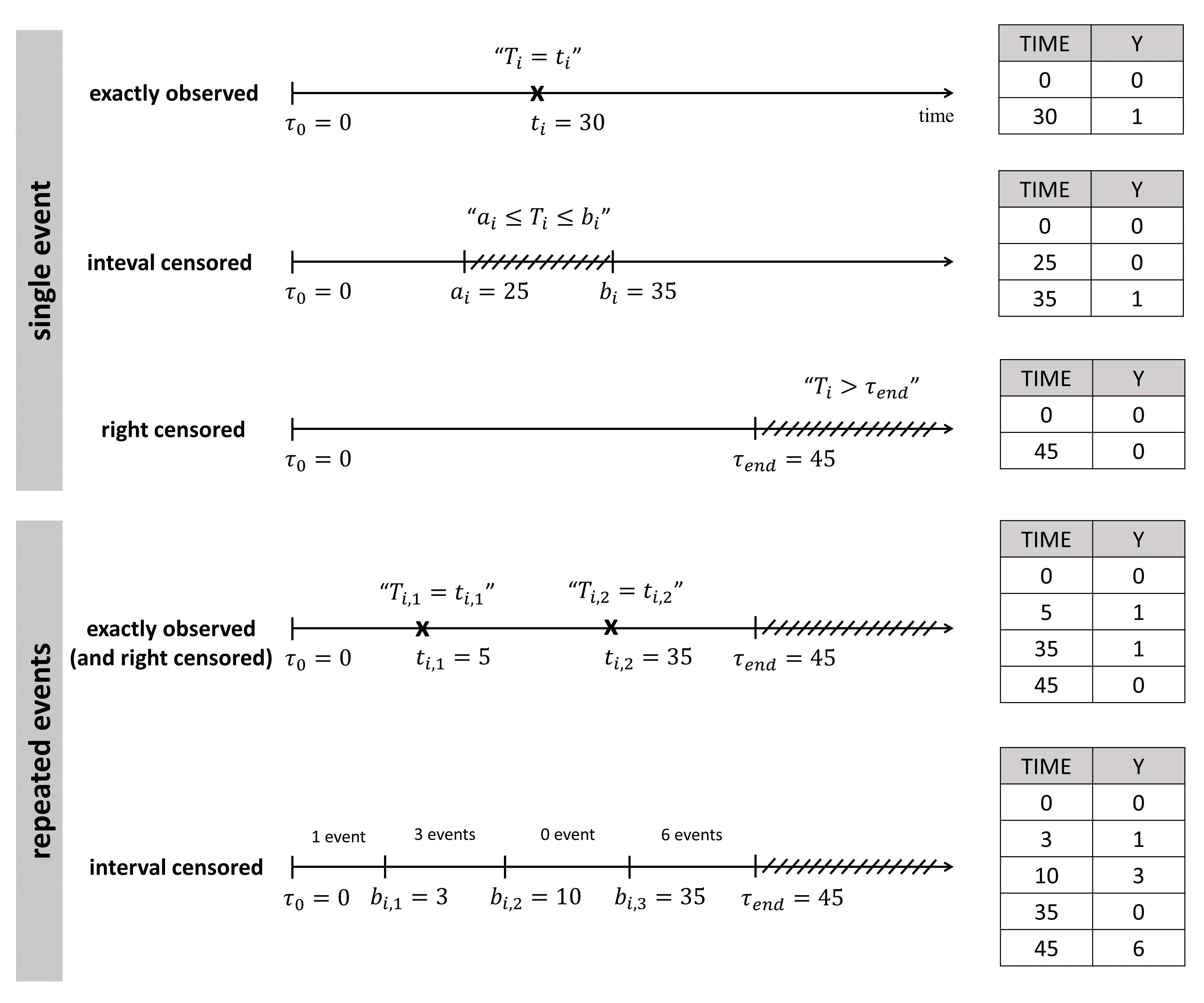
For instance for single events, exactly observed (with or without right censoring), one must indicate the start time of the observation period (Y=0), and the time of event (Y=1) or the time of the end of the observation period if no event has occurred (Y=0). In the following example:
ID TIME Y
1   0   0
1  34   1
2   0   0
2  80   0
the observation period lasts from starting time t=0 to the final time t=80. For individual 1, the event is observed at t=34, and for individual 2, no event is observed during the period. Thus it is noticed that at the final time (t=80), no event had occurred. Using absolute times instead of duration, we could equivalently write:
ID TIME Y
1  20   0
1  54   1
2  33   0
2  113  0
The duration between start time and event (or end of the observation period) are the same as before, but this time we record the day at which the patients enter the study and the days at which they have events or leave the study. Different patients may enter the study at different times.
Single event
To begin with, we will consider a one-off event. Depending on the application, the length of time to this event may be called the survival time (until death, for instance), failure time (until hardware fails), and so on. In general, we simply say “time-to-event”. The random variable representing the time-to-event for subject i is typically written Ti.
Single event exactly observed or right censored
- tte1_project (data = tte1_data.txt , model=lib:exponential_model_singleEvent.txt)
The event time may be exactly observed at time \(t_i\), but if we assume that the trial ends at time \(t_{\text{stop}}\), the event may happen after the end. This is “right censoring”. Here, Y=0 at time t means that the event happened after t and Y=1 means that the event happened at time t. The rows with t=0 are included to show the trial start time \(t_{\text{start}}=0\):
By clicking on the button Observed data, it is possible to display the Kaplan Meier plot (i.e. the empirical survival function) before fitting any model:
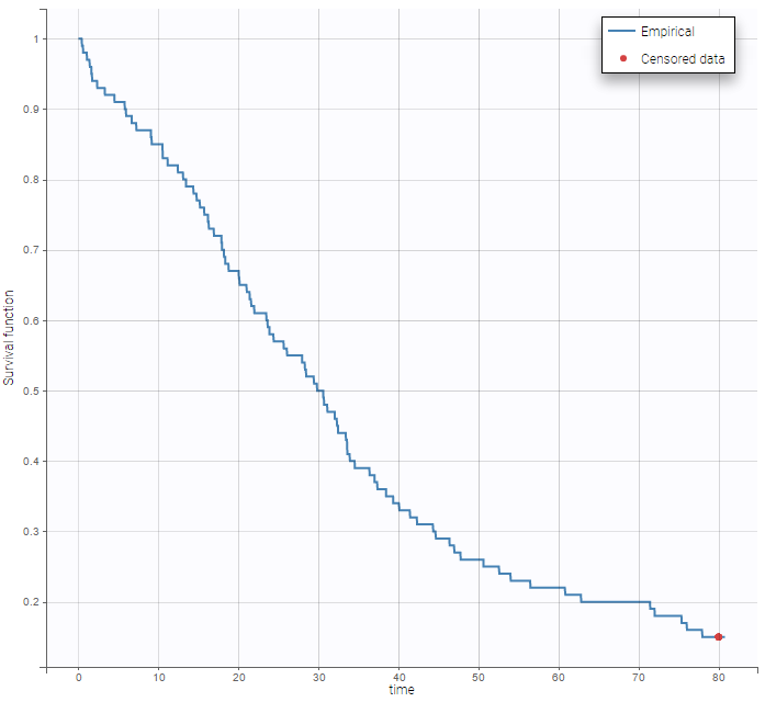
A very basic model with constant hazard is used for this data:
[LONGITUDINAL]
input = Te

EQUATION:
h = 1/Te

DEFINITION:
Event = {type=event, maxEventNumber=1, hazard=h}

OUTPUT:
output = {Event}
Here, Te is the expected time to event. Specification of the maximum number of events is required both for the estimation procedure and for the diagnosis plots based on simulation, such as the predicted interval for the Kaplan Meier plot which is obtained by Monte Carlo simulation:
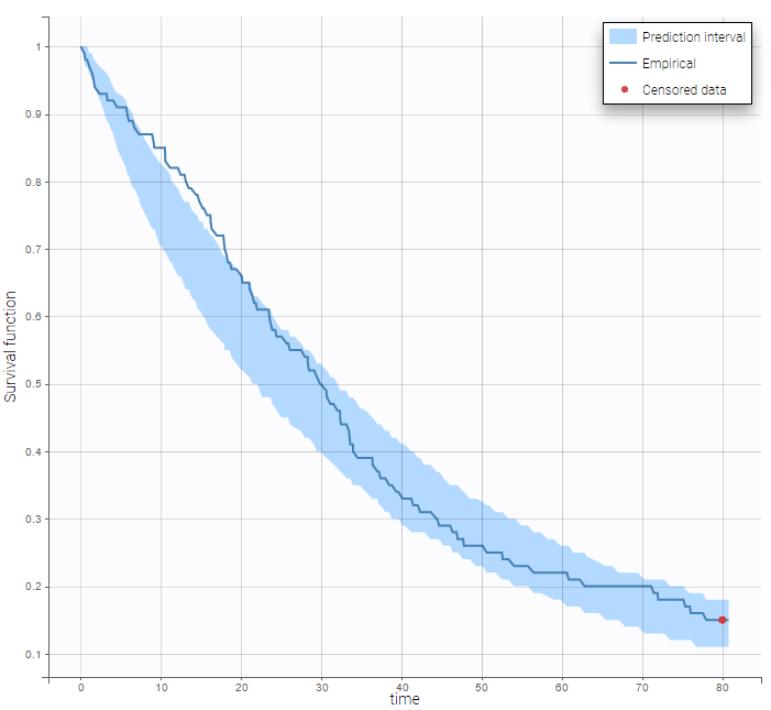
Single event interval censored or right censored
- tte2_project (data = tte2_data.txt , model=exponentialIntervalCensored_model.txt)
We may know the event has happened in an interval \(I_i\) but not know the exact time \(t_i\). This is interval censoring. Here, Y=0 at time t means that the event happened after t and Y=1 means that the event happened before time t.
Event for individual 1 happened between t=10 and t=15. No event was observed until the end of the experiment (t=100) for individual 5. We use the same basic model, but we now need to specify that the events are interval censored:
[LONGITUDINAL]
input = Te

EQUATION:
h = 1/Te

DEFINITION:
Event = {type=event, maxEventNumber=1, eventType=intervalCensored, hazard = h
         intervalLength=5     ; used for the plots (not mandatory)
}

OUTPUT:
output = Event
Repeated events
Sometimes, an event can potentially happen again and again, e.g., epileptic seizures, heart attacks. For any given hazard function h, the survival function S for individual i now represents the survival since the previous event at \(t_{i,j-1}\), given here in terms of the cumulative hazard from \(t_{i,j-1}\) to \(t_{i,j}\):
$$S(t_{i,j} | t_{i,j-1}; \psi_i) = \mathbb{P}(T_{i,j} > t_{i,j} | T_{i,j-1} = t_{i,j-1}; \psi_i) = \exp(-\int_{t_{i,j-1}}^{t_{i,j}}h(t,\psi_i) dt)$$
Repeated events exactly observed or right censored
- tte3_project (data = tte3_data.txt , model=lib:exponential_model_repeatedEvents.txt)
A sequence of \(n_i\) event times is precisely observed before \(t_{\text{stop}} = 200\): We can then display the Kaplan Meier plot for the first event and the mean number of events per individual:

After fitting the model, prediction intervals for these two curves can also be displayed on the same graph as on the following
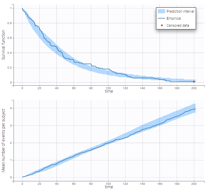
Repeated events interval censored or right censored
- tte4_project (data = tte4_data.txt , model=exponentialIntervalCensored_repeated_model.txt)
We do not know the exact event times, but the number of events that occurred for each individual in each interval of time.
User defined likelihood function for time-to-event data
- weibullRTTE (data = weibull_data.txt , model=weibullRTTE_model.txt)
A Weibull model is used in this example:
[LONGITUDINAL]
input = {lambda, beta}

EQUATION:
h = (beta/lambda)*(t/lambda)^(beta-1)

DEFINITION:
Event = {type=event, hazard=h, eventType=intervalCensored,
         intervalLength=5}

OUTPUT:
output = Event
- weibullCount (data = weibull_data.txt , model=weibullCount_model.txt)
Instead of defining the data as events, it is possible to consider the data as count data: indeed, we count the number of events per interval. An additional column with the start of the interval is added in the data file and defined as a regression variable. We then use a model for count data (see rtteWeibullCount_model.txt).
3.4.2.Count data model
- Introduction
- Formatting of count data in the MonolixSuite
- Count data with constant distribution over time
- Count data with time varying distribution
Objectives: learn how to implement a model for count data.
Projects: count1a_project, count1a_project, count1a_project, count2_project
Introduction
Longitudinal count data is a special type of longitudinal data that can take only nonnegative integer values {0, 1, 2, …} that come from counting something, e.g., the number of seizures, hemorrhages or lesions in each given time period . In this context, data from individual j is the sequence \(y_i=(y_{ij},1\leq j \leq n_i)\) where \(y_{ij}\) is the number of events observed in the jth time interval \(I_{ij}\).
Count data models can also be used for modeling other types of data such as the number of trials required for completing a given task or the number of successes (or failures) during some exercise. Here, \(y_{ij}\) is either the number of trials or successes (or failures) for subject i at time \(t_{ij}\). For any of these data types we will then model \(y_i=(y_{ij},1 \leq j \leq n_i)\) as a sequence of random variables that take their values in {0, 1, 2, …}. If we assume that they are independent, then the model is completely defined by the probability mass functions \(\mathbb{P}(y_{ij}=k)\) for \(k \geq 0\) and \(1 \leq j \leq n_i\). Here, we will only consider parametric distributions for count data.
Formatting of count data in the MonolixSuite
Count data can only take non-negative integer values that come from counting something, e.g., the number of trials required for completing a given task. The task can for instance be repeated several times and the individual’s performance followed. In the following data set:
ID TIME Y
1 0 10
1 24 6
1 48 5
1 72 2
10 trials are necessary the first day (t=0), 6 the second day (t=24), etc. Count data can also represent the number of events happening in regularly spaced intervals, e.g the number of seizures every week. If the time intervals are not regular, the data may be considered as repeated time-to-event interval censored, or the interval length can be given as regressor to be used to define the probability distribution in the model.
One can see the epilepsy attacks data set for a more practical example.
Modling count data in the MonolixSuite
Link to the detailed description of the library of count models integrated within Monolix.
Count data with constant distribution over time
- count1a_project (data = ‘count1_data.txt’, model = ‘count_library/poisson_mlxt.txt’)
A Poisson model is used for fitting the data:
[LONGITUDINAL]
input = lambda

DEFINITION:
Y = {type = count,  log(P(Y=k)) = -lambda + k*log(lambda) - factln(k) }

OUTPUT:
output = Y
Residuals for noncontinuous data reduce to NPDEs. We can compare the empirical distribution of the NPDEs with the distribution of a standardized normal distribution either with the pdf (top) or the cdf (bottom):
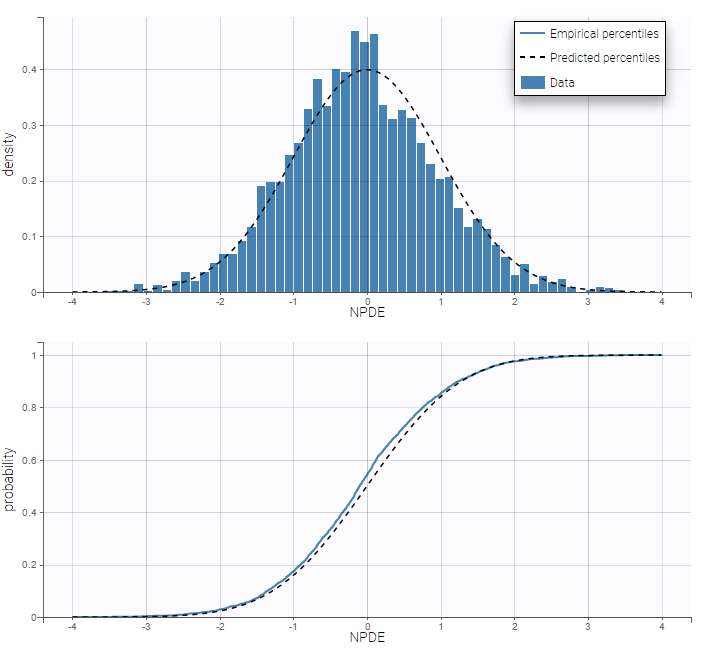
VPCs for count data compare the observed and predicted frequencies of the categorized data over time:
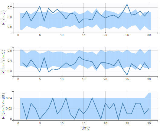
- count1b_project (data = ‘count1_data.txt’, model = ‘count_library/poissonMixture_mlxt.txt’)
A mixture of two Poisson distributions is used to fit the same data. For that, we define the probability of k occurrences as the weigthed sum of two Poisson distributions with two expected numbers of occurrences lambda1 and lambda2. The structural model file writes
[LONGITUDINAL]
input = {lambda1, alpha, mp}

EQUATION:
lambda2 = (1+alpha)*lambda1

DEFINITION:
Y = { type = count,
       P(Y=k) = mp*exp(-lambda1 + k*log(lambda1) - factln(k)) + (1-mp)*exp(-lambda2 + k*log(lambda2) - factln(k))
}

OUTPUT:
output = Y
Thus, the parameter alpha has to be strictly positive to ensure different expected number of occurrences in the two poisson distributions and mp has to be in [0, 1] to ensure the probability is correctly defined. Thus those parameters should be defined with lognormal and probitnormal distribution respectively as shown on the following figure.

We see on the VPC below that the data set is well modeled using this mixture of Poisson distributions.
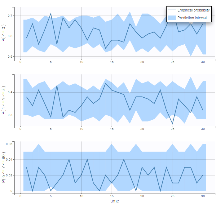
In addition, we can compute the prediction distribution of the modalities as on the following figure
Count data with time varying distribution
- count2_project (data = ‘count2_data.txt’, model = ‘count_library/poissonTimeVarying_mlxt.txt’)
The distribution of the data changes with time in this example:
We then use a Poisson distribution with a time varying intensity:
[LONGITUDINAL]
input =  {a,b}

EQUATION:
lambda= a*exp(-b*t)

DEFINITION:
y = {type=count, P(y=k)=exp(-lambda)*(lambda^k)/factorial(k)}

OUTPUT:
output = y
This model seems to fit the data very well:
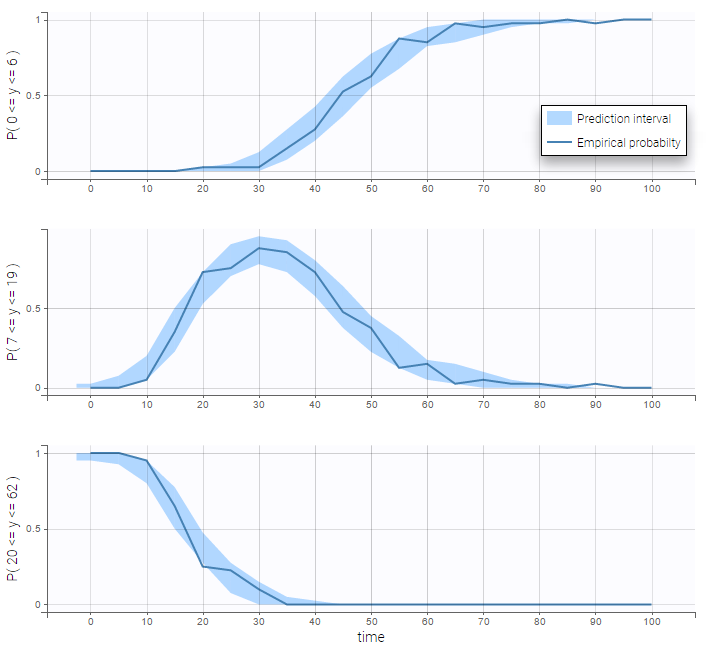
3.4.3.Categorical data model
- Introduction
- Formatting of categorical data in the MonolixSuite
- Ordered categorical data
- Ordered categorical data with regression variables
- Discrete-time Markov chain
- Continuous-time Markov chain
Objectives: learn how to implement a model for categorical data, assuming either independence or a Markovian dependence between observations.
Projects: categorical1_project, categorical2_project, markov0_project, markov1a_project, markov1b_project, markov1c_project, markov2_project, markov3a_project, markov3b_project
Introduction
Assume now that the observed data takes its values in a fixed and finite set of nominal categories \(\{c_1, c_2,\ldots , c_K\}\). Considering the observations \((y_{ij},\, 1 \leq j \leq n_i)\) for any individual \(i\) as a sequence of conditionally independent random variables, the model is completely defined by the probability mass functions \(\mathbb{P}(y_{ij}=c_k | \psi_i)\) for \(k=1,\ldots, K\) and \(1 \leq j \leq n_i\). For a given (i,j), the sum of the K probabilities is 1, so in fact only K-1 of them need to be defined. In the most general way possible, any model can be considered so long as it defines a probability distribution, i.e., for each k, \(\mathbb{P}(y_{ij}=c_k | \psi_i) \in [0,1]\), and \(\sum_{k=1}^{K} \mathbb{P}(y_{ij}=c_k | \psi_i) =1\). Ordinal data further assumed that the categories are ordered, i.e., there exists an order \(\prec\) such that
$$c_1 \prec c_2,\prec \ldots \prec c_K $$
We can think, for instance, of levels of pain (low \(\prec\) moderate \(\prec\) severe) or scores on a discrete scale, e.g., from 1 to 10. Instead of defining the probabilities of each category, it may be convenient to define the cumulative probabilities \(\mathbb{P}(y_{ij} \preceq c_k | \psi_i)\) for \(k=1,\ldots ,K-1\), or in the other direction: \(\mathbb{P}(y_{ij} \succeq c_k | \psi_i)\) for \(k=2,\ldots, K\). Any model is possible as long as it defines a probability distribution, i.e., it satisfies
$$0 \leq \mathbb{P}(y_{ij} \preceq c_1 | \psi_i) \leq \mathbb{P}(y_{ij} \preceq c_2 | \psi_i)\leq \ldots \leq \mathbb{P}(y_{ij} \preceq c_K | \psi_i) =1 .$$
It is possible to introduce dependence between observations from the same individual by assuming that \((y_{ij},\,j=1,2,\ldots,n_i)\) forms a Markov chain. For instance, a Markov chain with memory 1 assumes that all that is required from the past to determine the distribution of \(y_{ij}\) is the value of the previous observation \(y_{i,j-1}\)., i.e., for all \(k=1,2,\ldots ,K\),
$$\mathbb{P}(y_{ij} = c_k\,|\,y_{i,j-1}, y_{i,j-2}, y_{i,j-3},\ldots,\psi_i) = \mathbb{P}(y_{ij} = c_k | y_{i,j-1},\psi_i)$$
Formatting of categorical data in the MonolixSuite
In case of categorical data, the observations at each time point can only take values in a fixed and finite set of nominal categories. In the data set, the output categories must be coded as integers, as in the following example:
ID TIME Y
1 0.5 3
1 1 0
1 1.5 2
1 2 2
1 2.5 3
One can see the respiratory status data set and the warfarin data set for example for more practical examples on a categorical and a joint continuous and categorical data set respectively.
Ordered categorical data
- categorical1_project (data = ‘categorical1_data.txt’, model = ‘categorical1_model.txt’)
In this example, observations are ordinal data that take their values in {0, 1, 2, 3}:
- Cumulative odds ratio are used in this example to define the model
$$\textrm{logit}(\mathbb{P}(y_{ij} \leq k))= \log \left( \frac{\mathbb{P}(y_{ij} \leq k)}{1 – \mathbb{P}(y_{ij} \leq k )} \right)$$
where
$$\begin{array}{ccl} \text{logit}(\mathbb{P}(y_{ij} \leq 0)) &=& \theta_{i,1}\\ \text{logit}(\mathbb{P}(y_{ij} \leq 1)) &=& \theta_{i,1}+\theta_{i,2}\\ \text{logit}(\mathbb{P}(y_{ij} \leq 2)) &=& \theta_{i,1}+\theta_{i,2}+\theta_{i,3}\end{array}$$
This model is implemented in categorical1_model.txt:
[LONGITUDINAL]
input = {th1, th2, th3}

DEFINITION:
level = { type = categorical,  categories = {0, 1, 2, 3},
  logit(P(level<=0)) = th1
  logit(P(level<=1)) = th1 + th2
  logit(P(level<=2)) = th1 + th2 + th3
}
A normal distribution is used for \(\theta_{1}\), while log-normal distributions for \(\theta_{2}\) and \(\theta_{3}\) ensure that these parameters are positive (even without variability). Residuals for noncontinuous data reduce to NPDE’s. We can compare the empirical distribution of the NPDE’s with the distribution of a standardized normal distribution:
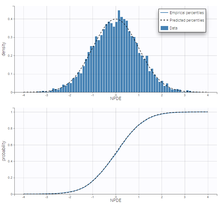
VPC’s for categorical data compare the observed and predicted frequencies of each category over time:
The prediction distribution can also be computed by Monte-Carlo:

Ordered categorical data with regression variables
- categorical2_project (data = ‘categorical2_data.txt’, model = ‘categorical2_model.txt’)
A proportional odds model is used in this example, where PERIOD and DOSE are used as regression variables (i.e. time-varying covariates)
Discrete-time Markov chain
If observation times are regularly spaced (constant length of time between successive observations), we can consider the observations \((y_{ij},j=1,2,\ldots,n_i)\) to be a discrete-time Markov chain.
- markov0_project (data = ‘markov1a_data.txt’, model = ‘markov0_model.txt’)
In this project, states are assumed to be independent and identically distributed:
\( \mathbb{P}(y_{ij} = 1) = 1 – \mathbb{P}(y_{ij} = 2) = p_{i,1} \)
Observations in markov1a_data.txt take their values in {1, 2}.
- markov1a_project (data = ‘markov1a_data.txt’, model = ‘markov1a_model.txt’)
Here,
\(\begin{aligned}\mathbb{P}(y_{i,j} = 1 | y_{i,j-1} = 1) = 1 – \mathbb{P}(y_{i,j} = 2 | y_{i,j-1} = 1) = p_{i,11}\\ \mathbb{P}(y_{i,j} = 1 | y_{i,j-1} = 2) = 1 – \mathbb{P}(y_{i,j} = 2 | y_{i,j-1} = 2) = p_{i,12} \end{aligned}\)
[LONGITUDINAL]
input = {p11, p21}
DEFINITION:
State = {type = categorical,  categories = {1,2},  dependence = Markov
  P(State=1|State_p=1) = p11
  P(State=1|State_p=2) = p21
}
The distribution of the initial state is not defined in the model, which means that, by default,
\( \mathbb{P}(y_{i,1} = 1) = \mathbb{P}(y_{i,1} = 2) = 0.5 \)
- markov1b_project (data = ‘markov1b_data.txt’, model = ‘markov1b_model.txt’)
The distribution of the initial state, \(p = \mathbb{P}(y_{i,1} = 1)\), is estimated in this example
DEFINITION:
State = {type = categorical,  categories = {1,2},  dependence = Markov
  P(State_1=1)= p
  P(State=1|State_p=1) = p11
  P(State=1|State_p=2) = p21
}
- markov3a_project (data = ‘markov3a_data.txt’, model = ‘markov3a_model.txt’)
Transition probabilities change with time in this example. We then define time varying transition probabilities in the model:
[LONGITUDINAL]
input = {a1, b1, a2, b2}
EQUATION:
lp11 = a1 + b1*t/100
lp21 = a2 + b2*t/100
DEFINITION:
State = {type = categorical, categories = {1,2}, dependence = Markov
  logit(P(State=1|State_p=1)) = lp11
  logit(P(State=1|State_p=2)) = lp21
}
- markov2_project (data = ‘markov2_data.txt’, model = ‘markov2_model.txt’)
Observations in markov2_data.txt take their values in {1, 2, 3}. Then, 6 transition probabilities need to be defined in the model.
Continuous-time Markov chain
The previous situation can be extended to the case where time intervals between observations are irregular by modeling the sequence of states as a continuous-time Markov process. The difference is that rather than transitioning to a new (possibly the same) state at each time step, the system remains in the current state for some random amount of time before transitioning. This process is now characterized by transition rates instead of transition probabilities:
\( \mathbb{P}(y_{i}(t+h) = k,|,y_{i}(t)=\ell , \psi_i) = h \rho_{\ell k}(t,\psi_i) + o(h),\qquad k \neq \ell .\)
The probability that no transition happens between \(t\) and \(t+h\) is
\( \mathbb{P}(y_{i}(s) = \ell, \forall s\in(t, t+h) | y_{i}(t)=\ell , \psi_i) = e^{h , \rho_{\ell \ell}(t,\psi_i)} .\)
Furthermore, for any individual i and time t, the transition rates \((\rho_{\ell,k}(t, \psi_i))\) satisfy for any \(1\leq \ell \leq K\),
\( \sum_{k=1}^K \rho_{\ell k}(t, \psi_i) = 0\)
Constructing a model therefore means defining parametric functions of time \((\rho_{\ell,k})\) that satisfy this condition.
- markov1c_project (data = ‘markov1c_data.txt’, model = ‘markov1c_model.txt’)
Observation times are irregular in this example. Then, a continuous time Markov chain should be used in order to take into account the Markovian dependence of the data:
DEFINITION:
State = { type = categorical,  categories = {1,2}, dependence = Markov
  transitionRate(1,2) = q12
  transitionRate(2,1) = q21
}
- markov3b_project (data = ‘markov3b_data.txt’, model = ‘markov3b_model.txt’)
Time varying transition rates are used in this example.
3.4.4.Joint models for non continuous outcomes
- Joint model for continuous PK and categorical PD data
- Joint model for continuous PK and count PD data
- Joint model for continuous PK and time-to-event data
Objectives: learn how to implement a joint model for continuous and non continuous data.
Projects: warfarin_cat_project, PKcount_project, PKrtte_project
Joint model for continuous PK and categorical PD data
- warfarin_cat_project (data = ‘warfarin_cat_data.txt’, model = ‘PKcategorical1_model.txt’)
In this example, the original PD data has been recorded as 1 (Low), 2 (Medium) and 3 (High).
More details about the data
International Normalized Ratio (INR) values are commonly used in clinical practice to target optimal warfarin therapy. Low INR values (<2) are associated with high blood clot risk and high ones (>3) with high risk of bleeding, so the targeted value of INR, corresponding to optimal therapy, is between 2 and 3.
Prothrombin complex activity is inversely proportional to the INR. We can therefore associate the three ordered categories for the INR to three ordered categories for PCA: Low PCA values if PCA is less than 33% (corresponding to INR>3), medium if PCA is between 33% and 50% (INR between 2 and 3) and high if PCA is more than 50% (INR<2).
The column dv contains both the PK and the new categorized PD measurements. Instead of modeling the original PD data, we can model the probabilities of each of these categories, which have direct clinical interpretations. The model is still a joint PKPD model since this probability distribution is expected to depend on exposure, i.e., the plasmatic concentration predicted by the PK model. We introduce an effect compartment to mimic the effect delay. Let \(y_{ij}^{(2)}\) be the PCA level for patient i at time \(t_{ij}^{(2)}\). We can then use a proportional odds model for modeling this categorical data:
$$\begin{array}{ccl}\text{logit} \left(\mathbb{P}(y_{ij}^{(2)} \leq 1 | \psi_i)\right) &= &\alpha_{i} + \beta_{i} Ce(t_{ij}^{(2)},\phi_i^{(1)}) \\ \text{logit} \left(\mathbb{P}(y_{ij}^{(2)} \leq 2 | \psi_i)\right) &=& \alpha_{i} + \gamma_{i} + \beta_{i}Ce(t_{ij}^{(2)},\phi_i^{(1)}) \\ \text{logit} \left(\mathbb{P}(y_{ij}^{(2)} \leq 3 | \psi_i)\right) &= & 1,\end{array}$$
where \(C_e(t,\phi_i^{(1)})\) is the predicted concentration of warfarin in the effect compartment at time t for patient i with PK parameters \(\phi_i^{(1)}\). This model defines a probability distribution for \(y_{ij}\) if \(\gamma_i\geq 0\).
If \(\beta_i>0\), the probability of low PCA at time \(t_{ij}^{(2)}\) (\(y_{ij}^{(2)}=1\)) increases along with the predicted concentration \(Ce(t_{ij}^{(2)},\phi_i^{(1)})\). The joint model is implemented in the model file PKcategorical1_model.txt
[LONGITUDINAL]
input = {Tlag, ka, V, Cl, ke0, alpha, beta, gamma}

EQUATION:
{Cc,Ce} = pkmodel(Tlag,ka,V,Cl,ke0)
lp1 = alpha + beta*Ce
lp2 = lp1+ gamma         ; gamma >= 0

DEFINITION:
Level = {type=categorical, categories={1,2,3}
    logit(P(Level<=1)) = lp1
    logit(P(Level<=2)) = lp2
}
OUTPUT:
output = {Cc, Level}
See Categorical data model for more details about categorical data models.
Joint model for continuous PK and count PD data
- PKcount_project (data = ‘PKcount_data.txt’, model = ‘PKcount1_model.txt’)
The data file used for this project is PKcount_data.txt where the PK and the count PD measurements are simulated. We use a Poisson distribution for the count data, assuming that the Poisson parameter is function of the predicted concentration. For any individual i, we have
$$\lambda_i(t) = \lambda_{0,i} \left( 1 – \frac{Cc_i(t)}{Cc_i(t) + IC50_i} \right)$$
where \(Cc_i(t)\) is the predicted concentration for individual i at time t and
$$ \log\left(P(y_{ij}^{(2)} = k)\right) = -\lambda_i(t_{ij}) + k\,\log(\lambda_i(t_{ij})) – \log(k!)$$
The joint model is implemented in the model file PKcount1_model.txt
[LONGITUDINAL]
input = {ka, V, Cl, lambda0, IC50}

EQUATION:
Cc = pkmodel(ka,V,Cl)
lambda=lambda0*(1 - Cc/(IC50+Cc))

DEFINITION:
Seizure = {type = count,
           log(P(Seizure=k)) = -lambda + k*log(lambda) - factln(k)
}

OUTPUT:
output = {Cc,Seizure}
See Count data model for more details about count data models.
Joint model for continuous PK and time-to-event data
- PKrtte_project (data = ‘PKrtte_data.txt’, model = ‘PKrtteWeibull1_model.txt’)
The data file used for this project is PKrtte_data.txt where the PK and the time-to-event data are simulated. We use a Weibull model for the events count data, assuming that the baseline is function of the predicted concentration. For any individual i, we define the hazard function as
$$h_i(t) = \gamma_{i} Cc_i(t) t^{\beta-1}$$
where \(Cc_i(t)\) is the predicted concentration for individual i at time t. The joint model is implemented in the model file PKrtteWeibull1_model.txt
[LONGITUDINAL]
input  = {ka, V, Cl, gamma, beta}

EQUATION:
Cc = pkmodel(ka, V, Cl)
if t<0.1
  haz = 0
else
  haz = gamma*Cc*(t^(beta-1))
end

DEFINITION:
Hemorrhaging  = {type=event, hazard=haz}

OUTPUT:
output = {Cc, Hemorrhaging}
See Time-to-event data model for more details about time-to-event data models.
3.5.Extensions
3.5.1.Using a scale factor
By default the models from the library do not include a scale factor. Units of the estimated parameters will depend on the units of the data set. For instance:
- Concentration in mg/L, amount in mg, time in hours => volumes are in L and clearances in L/h
- Concentration in ng/mL, amount in mg, time in minutes => volume are in 10^3 L and clearances in 10^3 L/min
The files from the library can easily be modified to include a scale factor:
Step 1: load a model from the library.
Step 2: in the “Structural model” tab, click “Open in editor”.
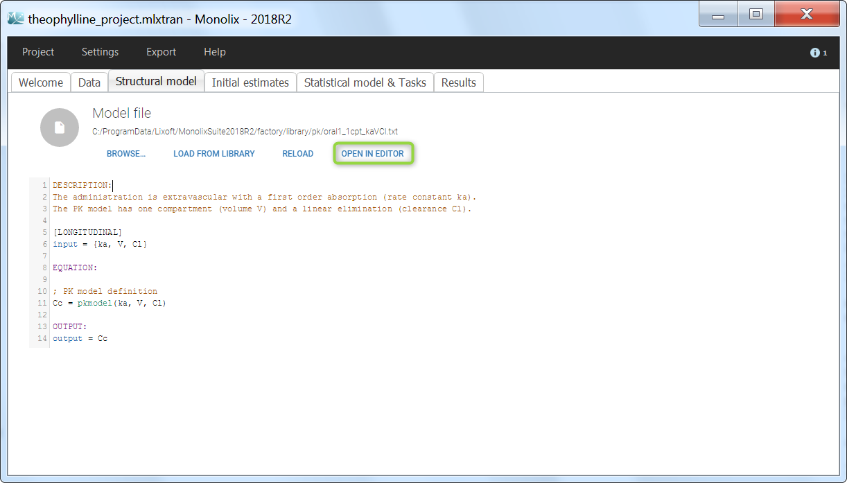
Step 3: add a scaling of the concentration. If the dose is in mg and I want the volume in L, then the concentration Cc will be in mg/L. If my observations in the data set are in ng/mL (i.e μg/L), I need to multiply Cc by 1000 (green highlight). Do not forget to output the scaled concentration instead of the original one (pink highlight).
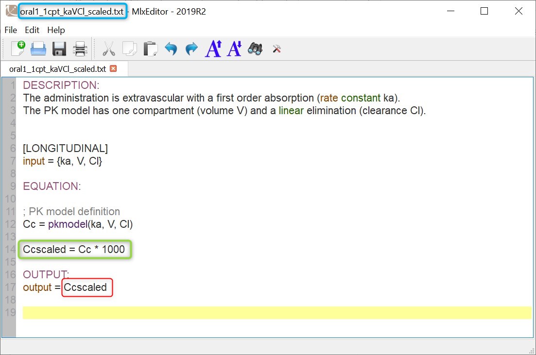
Step 4: save the file under a new name (to avoid overwriting the library model files).
Step 5: load the saved model file.
3.5.2.Using regression variables
- Introduction
- Regressor definition in a data set
- Continuous regression variables
- Categorical regression variables
Objectives: learn how to define and use regression variables (time varying covariates).
Projects: reg1_project, reg2_project
Introduction
A regression variable is a variable x which is a given function of time, which is not defined in the model but which is used in the model. x is only defined at some time points \(t_1, t_2, \ldots, t_m\) (possibly different from the observation time points), but x is a function of time that should be defined for any t (if is used in an ODE for instance, or if a prediction is computed on a fine grid). Then, Mlxtran defines the function x by interpolating the given values \((x_1, x_2, \ldots, x_m)\). In the current version of Mlxtran, interpolation is performed by using the last given value:
\( x(t) = x_j \quad~~\text{for}~~t_j \leq t < t_{j+1} \)
The way to introduce it in the Mlxtran longitudinal model is defined here.
Regressor definition in a data set
It is possible to have in a data set one or several columns with column-type REGRESSOR. Within a given subject-occasion, string “.” will be interpolated (last value carried forward interpolation is used) for observation and dose-lines. Lines with no observation and no dose but with regressor values are also taken into account by Monolix for regressor interpolation.
Several points have to be noticed:
- The name of the regressor in the data set and the name of the regressor used in the longitudinal model do not need to be identical.
- If there are several regressors, the mapping will be done by order of definition.
- Regressors can only be used in the longitudinal model.
Continuous regression variables
- reg1_project (data = reg1_data.txt , model=reg1_model.txt)
We consider a basic PD model in this example, where some concentration values are used as a regression variable. The data set is defined as follows
[LONGITUDINAL]
input = {Emax, EC50, Cc}
Cc    = {use=regressor}

EQUATION:
E = Emax*Cc/(EC50 + Cc)

OUTPUT:
output = E
As explained in the previous subsection, there is no name correspondance between the regressor in the data set and the regressor in the model file. Thus, in that case, the values of Cc with respect to time will be taken from the y1 column.
In addition, in that case, the predicted effect is therefore piece wise constant because
- the regressor interpolation is performed by using the last given value, and then Cc is piece wise constant.
- The effect model is direct with respect to the concentration.
Thus, it changes at the time points where concentration values are provided:

Categorical regression variables
- reg2_project (data = reg2_data.txt , model=reg2_model.txt)
The variable \(z_{ij}\) takes its values in {1, 2} in this example and represents the state of individual i at time \(t_{ij}\). We then assume that the observed data \(y_{ij}\) has a Poisson distribution with parameter lambda1 if \(z_{ij}=1\) and parameter lambda2 if \(z_{ij}=2\). z is known in this example: it is then defined as a regression variable in the model:
[LONGITUDINAL]
input = {lambda1, lambda2, z}
z = {use=regressor}

EQUATION:
if z==0
   lambda=lambda1
else
   lambda=lambda2
end

DEFINITION:
y = {type=count,
     log(P(y=k)) = -lambda + k*log(lambda) - factln(k)
}

OUTPUT:
output = y
3.5.3.Delayed differential equations
- Ordinary differential equations based model
- Don’t forget the initial conditions!
- Delayed differential equations based model
Objectives: learn how to implement a model with ordinary differential equations (ODE) and delayed differential equations (DDE).
Projects: tgi_project, seir_project
Ordinary differential equations based model
- tgi_project (data = tgi_data.txt , model = tgi_model.txt)
Here, we consider the tumor growth inhibition (TGI) model proposed by Ribba et al. (Ribba, B., Kaloshi, G., Peyre, M., Ricard, D., Calvez, V., Tod, M., . & Ducray, F., *A tumor growth inhibition model for low-grade glioma treated with chemotherapy or radiotherapy*. Clinical Cancer Research, 18(18), 5071-5080, 2012.). This model is defined by a set of ordinary differential equations
 \\\frac{dP_T}{dt} &= \lambda P_T(t)(1- P^{\star}(t)/K) + k_{QPP}Q_P(t) -k_{PQ} P_T(t) -\gamma \, k_{de} P_T(t)C(t) \\ \frac{dQ_T}{dt} &= k_{PK} P_T(t) -\gamma k_{de} Q_T(t)C(t) \\\frac{dQ_P}{dt} &= \gamma k_{de} Q_T(t)C(t) - k_{QPP} Q_P(t) -\delta_{QP} Q_P(t)\end{aligned}")
where  = P_T(t) + Q_T(t) + Q_P(t)")
 &= 0 \\ P_T(0) &= P_{T0} \\ Q_T(0) &= Q_0 \\ Q_P(0) &= 0 \end{aligned}")
This model (derivatives and initial conditions) can easily be implemented with Mlxtran:
DESCRIPTION: Tumor Growth Inhibition (TGI) model proposed by Ribba et al
A tumor growth inhibition model for low-grade glioma treated with chemotherapy or radiotherapy.
Clinical Cancer Research, 18(18), 5071-5080, 2012.

Variables
- PT: proliferative equiescent tissue
- QT: nonproliferative equiescent tissue
- QP: damaged quiescent cells
- C:  concentration of a virtual drug encompassing the 3 chemotherapeutic components of the PCV regimen

Parameters
- K      : maximal tumor size (should be fixed a priori)
- KDE    : the rate constant for the decay of the PCV concentration in plasma
- kPQ    : the rate constant for transition from proliferation to quiescence
- kQpP   : the rate constant for transfer from damaged quiescent tissue to proliferative tissue
- lambdaP: the rate constant of growth for the proliferative tissue
- gamma  : the rate of damages in proliferative and quiescent tissue
- deltaQP: the rate constant for elimination of the damaged quiescent tissue
- PT0    : initial proliferative equiescent tissue
- QT0    : initial nonproliferative equiescent tissue

[LONGITUDINAL]
input = {K, KDE, kPQ, kQpP, lambdaP, gamma, deltaQP, PT0, QT0}

PK:
depot(target=C)

EQUATION:
; Initial conditions
t0    = 0
C_0   = 0
PT_0  = PT0
QT_0  = QT0
QP_0  = 0

; Dynamical model
PSTAR   = PT + QT + QP
ddt_C   = -KDE*C
ddt_PT  = lambdaP*PT*(1-PSTAR/K) + kQpP*QP - kPQ*PT - gamma*KDE*PT*C
ddt_QT  = kPQ*PT - gamma*KDE*QT*C
ddt_QP  = gamma*KDE*QT*C - kQpP*QP - deltaQP*QP

OUTPUT:
output = PSTAR
Remark: t0, PT_0 and QT_0 are reserved keywords that define the initial conditions.
Then, the graphic of individual fits clearly shows that the tumor size is constant until 

Don’t forget the initial conditions!
- tgiNoT0_project (data = tgi_data.txt , model = tgiNoT0_model.txt)
The initial time t0 is not specified in this example. Since t0 is missing, Monolix uses the first time value encountered for each individual. If, for instance, the tumor size has not been computed before 5 for the individual fits, then t0=5 will be used for defining the initial conditions for this individual, which introduces a shift in the plot:

As defined here, the following rule applies
- When no starting time t0 is defined in the Mlxtran model for Monolix then by default t0 is selected to be equal to the first dose or the first observation, whatever comes first.
- If t0 is defined, a differential equation needs to be defined.
Conclusion: don’t forget to properly specify the initial conditions of a system of ODEs!
Delayed differential equations based model
A system of delay differential equations (DDEs) can be implemented in a block EQUATION of the section [LONGITUDINAL] of a script Mlxtran. Mlxtran provides the command delay(x,T) where x is a one-dimensional component and T is the explicit delay. Therefore, DDEs with a nonconstant past of the form
$$ \begin{array}{ccl} \frac{dx}{dt} &=& f(x(t),x(t-T_1), x(t-T_2), …), ~~\text{for}~~t \geq 0\ x(t) &=& x_0(t) ~~~~\text{for}~~\text{min}(T_k) \leq t \leq 0 \end{array} $$
can be solved. The syntax and rules are explained here.
- seir_project (data = seir_data.txt , model = seir_model.txt)
The model is a system of 4 DDEs and defined with the following mode:
DESCRIPTION: SEIR model, using delayed differential equations.
"An Epidemic Model with Recruitment-Death Demographics and Discrete Delays", Genik & van den Driessche (1999)
Decomposition of the total population into four epidemiological classes
S (succeptibles), E (exposed), I (infectious), and R (recovered)
The parameters corresponds to
- birthRate: the birth rate,
- deathRate: the natural death rate,
- infectionRate: the contact rate of infective individuals,
- recoveryRate: the rate of recovery,
- excessDeathRate: the excess death rate for infective individuals
There is a time delay in the model:
- tauImmunity: a temporary immunity delay
[LONGITUDINAL]
input = {birthRate, deathRate, infectionRate, recoveryRate, excessDeathRate, tauImmunity, tauLatency}
EQUATION:
; Initial conditions
t0 = 0
S_0 = 15
E_0 = 0
I_0 = 2
R_0 = 3
; Dynamical model
N = S + E + I + R
ddt_S = birthRate - deathRate*S - infectionRate*S*I/N + recoveryRate*delay(I,tauImmunity)*exp(-deathRate*tauImmunity)
ddt_E = infectionRate*S*I/N - deathRate*E - infectionRate*delay(S,tauLatency)*delay(I,tauLatency)*exp(-deathRate*tauLatency)/(delay(I,tauLatency)+delay(S,tauLatency)+delay(E,tauLatency)+delay(R,tauLatency))
ddt_I = -(recoveryRate+excessDeathRate+deathRate)*I + infectionRate*delay(S,tauLatency)*delay(I,tauLatency)*exp(-deathRate*tauLatency)/(delay(I,tauLatency)+delay(S,tauLatency)+delay(E,tauLatency)+delay(R,tauLatency))
ddt_R = recoveryRate*I - deathRate*R - recoveryRate*delay(I,tauImmunity)*exp(-deathRate*tauImmunity)
OUTPUT:
output = {S, E, I, R}
Introducing these delays allows to obtain nice fits for the 4 outcomes, including ")

Case studies
- 8.case_studies/arthritis_project
3.5.4.Outputs and Tables
Objectives: learn how to define outputs and create tables from the outputs of the model.
Projects: tgi_project, tgiWithTable_project
About the OUTPUT block
- tgi_project (data = ‘tgi_data.txt’ , model=’tgi_model.txt’)
We use the Tumor Growth Inhibition (TGI) model proposed by Ribba et al. in this example (Ribba, B., Kaloshi, G., Peyre, M., Ricard, D., Calvez, V., Tod, M., . & Ducray, F., A tumor growth inhibition model for low-grade glioma treated with chemotherapy or radiotherapy. Clinical Cancer Research, 18(18), 5071-5080, 2012.)
DESCRIPTION: Tumor Growth Inhibition (TGI) model proposed by Ribba et al
A tumor growth inhibition model for low-grade glioma treated with chemotherapy or radiotherapy.
Clinical Cancer Research, 18(18), 5071-5080, 2012.

Variables
- PT: proliferative equiescent tissue
- QT: nonproliferative equiescent tissue
- QP: damaged quiescent cells
- C:  concentration of a virtual drug encompassing the 3 chemotherapeutic components of the PCV regimen

Parameters
- K      : maximal tumor size (should be fixed a priori)
- KDE    : the rate constant for the decay of the PCV concentration in plasma
- kPQ    : the rate constant for transition from proliferation to quiescence
- kQpP   : the rate constant for transfer from damaged quiescent tissue to proliferative tissue
- lambdaP: the rate constant of growth for the proliferative tissue
- gamma  : the rate of damages in proliferative and quiescent tissue
- deltaQP: the rate constant for elimination of the damaged quiescent tissue
- PT0    : initial proliferative equiescent tissue
- QT0    : initial nonproliferative equiescent tissue

[LONGITUDINAL]
input = {K, KDE, kPQ, kQpP, lambdaP, gamma, deltaQP, PT0, QT0}

PK:
depot(target=C)

EQUATION:
; Initial conditions
t0    = 0
C_0   = 0
PT_0  = PT0
QT_0  = QT0
QP_0  = 0

; Dynamical model
PSTAR   = PT + QT + QP
ddt_C   = -KDE*C
ddt_PT  = lambdaP*PT*(1-PSTAR/K) + kQpP*QP - kPQ*PT - gamma*KDE*PT*C
ddt_QT  = kPQ*PT - gamma*KDE*QT*C
ddt_QP  = gamma*KDE*QT*C - kQpP*QP - deltaQP*QP

OUTPUT:
output = PSTAR
PSTAR is the tumor size predicted by the model. It is therefore used as a prediction for the observations in the project.
At the end of the scenario or of SAEM, individual predictions of the tumor size PSTAR are computed using the individual parameters available. Thus, individual predictions of the tumor size PSTAR are computed using both the conditional modes (indPred_mode), the conditional mean (indPred_mean), and the conditional means estimated during the last iterations of SAEM (indPred_SAEM) and saved in the table predictions.txt.
Notice that the population prediction is also proposed.

Remark: the same model file tgi_model.txt can be used with different tools, including Mlxplore or Simulx.
Add additional outputs in tables
- tgiWithTable_project (data = ‘tgi_data.txt’ , model=’tgiWithTable_model.txt’)
We can save in the tables additional variables defined in the model, such as PT, Q and QP for instance, by adding a block OUTPUT: in the model file:
OUTPUT:
output = PSTAR
table  = {PT, QT, QP}
An additional file tables.txt now includes the predicted values of these variables for each individual (columns PT_mean, QT_mean, QP_mean, PT_mode, QT_mode, QP_mode, PT_popPred, QT_popPred, QP_popPred, PT_popPred_medianCOV, QT_popPred_medianCOV, QP_popPred_medianCOV, PT_SAEM, QT_SAEM, and QP_SAEM.

Notice that only continuous variable are possible for variable in table.
Good to know: it is not allowed to do calculations directly in the output or table statement. The following example is not possible:
; not allowed:
OUTPUT:
output = {Cser+Ccsf}
It has to be replaced by:
EQUATION:
Ctot = Cser+Ccsf
OUTPUT:
output = {Ctot}
3.5.5.How to compute AUC using in Monolix and Mlxtran
Computing additional outputs such as AUC and Cmax in the structural model is possible but requires a particular syntax, because it is not possible to redefine a variable in Mlxtran. For example, it would not be possible to directly update the variable Cmax = Cc when Cc>Cmax. But it is possible to compute Cmax via an ODE, where Cmax increases like Cc at each time where Cc>Cmax. This page gives detailed examples for the AUC on full time interval or specific interval, Cmax, nadir, and other derived variables such as duration above a threshold.
Often the Area under the PK curve (AUC) is needed as an important PK metric to link with the pharmacodynamic effect. We show here how to:
- compute the AUC within the mlxtran model file
- output the AUC calculations for later analysis.
Calculation of the AUC can be done in the EQUATION section of the Mlxtran model. If a dataset contains the AUC observations, then the calculation in the EQUATION section can be used as an output in the output={} definition (matched to observations of the data set). Or it can be saved for post-treatment using table={}, as described here.
AUClast from t=0 to t=tlast
The following code is the basic implementation of the AUC for a 1-compartmental model with the absorption rate ka. It integrates the concentration profile from the start to the end of the observation period.
[LONGITUDINAL]
input = {ka, V, Cl}

PK:
Cc=pkmodel(ka,V,Cl)

EQUATION:
odeType=stiff
ddt_AUC = Cc

OUTPUT:
output = {Cc}
table  = {AUC}
AUC in a time interval
The following code computes the AUC between two time points t1 and t2. The idea is to compute the AUC_0_t1 and AUC_0_t2 using if/else statements and then do the difference between the two.
[LONGITUDINAL]
input = {ka, V, Cl}
PK:
depot(ka, target=Ac)

EQUATION:
odeType = stiff
useAnalyticalSolution=no

Cc = pkmodel(ka,V,Cl)

t1=24
t2=48
AUCt1_0 = 0
if(t < t1)
   dAUCt1 = Cc
else
   dAUCt1 = 0
end
ddt_AUCt1 = dAUCt1

AUCt2_0 = 0
if(t < t2)
   dAUCt2 = Cc
else
   dAUCt2 = 0
end
ddt_AUCt2 = dAUCt2

AUC_t1_t2 = AUCt2 - AUCt1

OUTPUT:
output = {Cc}
table  = {AUC_t1_t2}
Note that the t==tDose would not work because the integrator does not necessarily evaluate the time exactly at the times of doses. Thus the test t==tDose might not be tested at all during the computation.
Also note that, although partial AUC can be calculated by comparing time with the both boundaries in the if statement (e.g. if (t>20 and t<40)), this might not be the best practice when concentration is calculated using an analytical solution, because ODE solver used for calculating AUC could be deceived by AUC remaining 0 for a period of time and might increase the integration time step to a value larger than the difference between time boundaries.
Dose-interval AUC (AUCtau)
The following code compute the AUCtau for each dose interval. At each dose the AUC is reset to zero and the concentration is integrated until the next administration.
[LONGITUDINAL]
input = {ka, V, Cl}

PK:
Cc = pkmodel(ka,V,Cl)

; Reset the ODE variable AUCtau to zero each time there is a dose
empty(target=AUCtau)
EQUATION:
odeType=stiff
ddt_AUCtau = Cc

OUTPUT:
output = {Cc}
table = {AUCtau}
Computing the Cmax or nadir in the structural model
Cmax
Cmax can be calculated directly in the structural model by integrating the increase of the concentration. Alternatively, the Cmax can also be calculated in Simulx using the Outcomes&Endpoints tab.
Cmax for models with first-order absorption
The following example shows how to do it in case of a one-compartment model with first-order absorption and linear elimination. Absorption processes defined via the depot macro must be replaced by explciit ODEs, while the depot macro is used to add the dose as a bolus into the depot compartment.
[LONGITUDINAL]
input = {Cl, ka, V}

PK:
depot(target=Ad)

EQUATION:

; initial conditions
t_0  = 0
Ad_0 = 0
Ac_0 = 0

ddt_Ad = -ka*Ad
ddt_Ac = ka*Ad - k*Ac
Cc = Ac/V

; Calculation of Cmax
slope  = ka*Ad -k*Ac
Cmax_0 = 0
if slope > 0 && Cc > Cmax
   x = slope/V
else
   x = 0
end
ddt_Cmax = x
Cmax for model with bolus administration or infusion
If the dose is administered as bolus, it is necessary to add in the model a very short infusion. This prevents from the instantaneous increase of the concentration. The following example shows this situations in case of a three-compartments model with linear elimination. The duration of the “short infusion” can be adapted with respect to the time scale by modifying dT=0.1.
If the doses are administered via iv infusion, then dT=0.1 can be replaced by dT = inftDose, which reads the infusion duration from the data.
[LONGITUDINAL]
input = {Cl, V1, Q2, V2, Q3, V3}

EQUATION:

; Parameter transformations
V   = V1
k   = Cl/V1
k12 = Q2/V1
k21 = Q2/V2
k13 = Q3/V1
k31 = Q3/V3

; initial conditions
t_0  = 0
Ac_0 = 0
A2_0 = 0
A3_0 = 0

;short pseudo-infusion duration
dT = 0.1 ; use dT=inftDose if the administration is infusion: inftDose is the infusion duration from the last dose read from the data

; infusion input to Ac
if t < tDose+dT
   input = amtDose/dT ;amtDose is the last dose amount read from the data
else
   input = 0
end

dAc = input -k*Ac - k12*Ac - k13*Ac + k21*A2 + k31*A3
ddt_Ac = dAc
ddt_A2 = k12*Ac - k21*A2
ddt_A3 = k13*Ac - k31*A3
Cc = Ac/V

; Calculation of AUC
AUC_0 = 0
ddt_AUC = Cc

; Calculation of Cmax
Cmax_0 = 0
if dAc > 0 && Cc > Cmax
   x = dAc/V
else
   x = 0
end

ddt_Cmax = x

OUTPUT:
output = {Ac, Cc}
table  = {Cmax, AUC}
Cmax for models with transit compartments
The transit compartments defined via the depot() macro must be replaced by explicit ODEs. The amount in the last (nth) transit compartment is described via an analytical solution using the keyword amtDose to get the dose amount and (t-tDose) to get the time elapsed since the last dose. The calculation of Cmax then follows the same logic as for a first-order absorption.
[LONGITUDINAL]
input={F, Ktr, Mtt, ka, V, Cl}

EQUATION:
k = Cl/V
odeType=stiff

; transit model with explicit ODEs
n = max(0, Mtt*Ktr - 1)
An = F * amtDose * exp( n * log(Ktr*(t-tDose)) - factln(n) - Ktr * (t-tDose))

t_0 = 0
Aa_0 = 0
Ac_0 = 0

ddt_Aa = Ktr*An - ka*Aa
ddt_Ac = ka*Aa - k*Ac
Cc = Ac/V
; Calculation of Cmax
slope  = ka*Aa - k*Ac
Cmax_0 = 0
if slope > 0 && Cc > Cmax
   x = slope/V
else
   x = 0
end
ddt_Cmax = x

OUTPUT:
output = {Cc}
table = {Cmax}
Nadir
This example shows how to compute tumor size (variable TS) at time of nadir:
[LONGITUDINAL]
input = {ka, Vl, Cl, TS0, kge, kkill, lambda}
EQUATION:

odeType=stiff
Cc = pkmodel(ka, V, Cl)

; ODE system for tumor growth dynamics
t_0 = 0
TS_0 = TS0
TSDynamics = (kge*TS)-kkill*TS*Cc*exp(-lambda*t)
ddt_TS = TSDynamics

; ===== computing TS at nadir
if TSDynamics < 0 && TS < TS_atNadir
  x = TSDynamics
else
  x = 0
end
TS_atNadir_0 = TS0
ddt_TS_atNadir = x

OUTPUT:
output = {TS}
table = {TS_atNadir}
Here is an example of simulation for TS and TS_atNadir with a multiple dose schedule:
Time above a threshold
Here we compute the time that a variable C spends above some threshold, which could be a toxicity threshold for example. This piece of code comes in the structural model, after the dynamics of the variable C has already been defined.
TimeAboveThreshold_0 = 0
if C > Cthreshold
  xTime = 1
else
  xTime = 0
end
ddt_TimeAboveThreshold = xTime
Time since disease progression
In this full structural model example, tumor size TS is described with an exponential growth, and a constant treatment effect since time=0 with a log-kill killing hypothesis and a Claret exponential resistance term. Several additional variables are computed:
- TS_atNadir: the tumor size at the time of nadir,
- PC_from_Nadir: the percent change of TS between the time of nadir and the current time,
- DP: predicted disease progression status (1 if TS has increased more than >20% and >5-mm from last nadir, 0 otherwise),
- TDP: time since disease progression (duration since last time when DP is switched from 0 to 1)
[LONGITUDINAL]
input = {TS0, kge, kkill, lambda}

EQUATION:
odeType=stiff

;initial conditions:
;t_0 = 0 ;this should be uncommented if the initial time is 0 for all subjects
TS_0 = TS0

K = kkill*exp(-lambda*t)

;Saturation for TS at 1e12 to avoid infinite values
if TS>1e12
  TSDynamics = 0
  else
  if t<0 ; before treatment
    TSDynamics = (kge*TS)
  else ; after treatment
    TSDynamics = (kge*TS)-K*TS
  end
end

ddt_TS = TSDynamics

; Computing time to nadir (TS decreases after treatment start at time=0, then increases again because of resistance)
if TSDynamics<0
  x1=1
else
  x1=0
end
TimeToNadir_0=t0
ddt_TimeToNadir = x1 ; x1 is used as intermediate variable because it is not possible to define an ODE inside an if/else statement

; Computing TS at time of nadir
if TSDynamics < 0 & TS < TS_atNadir
  x2 = TSDynamics
else
  x2 = 0
end
TS_atNadir_0 = TS0
ddt_TS_atNadir = x2 ;

; Computing DP: predicted disease progression status at the previous visit (1 if TS has increased more than >20% and >5-mm from last nadir, 0 otherwise)
PC_from_Nadir = (TS/TS_atNadir-1)*100
if t>TimeToNadir & PC_from_Nadir > 20 & (TS-TS_atNadir) > 5
  DP = 1
else
  DP = 0
end

; Computing TDP = time since disease progression: duration since last time DP was switched from 0 to 1
if DP==1
  x3 = 1
else
  x3 = 0
end
TDP_0 = 0
ddt_TDP = x3

OUTPUT:
output = {TS}
table = {TS_atNadir, PC_from_Nadir, DP, TDP}
Simulx can be conveniently used to simulate each intermediate variable with typical parameters (the example model and Simulx project can be downloaded here):
4.Statistical Model
The statistical model tab in Monolix enables to define the statistical model and run estimation tasks.
The statistical model includes
- the observation model, which combines the error model and the distribution of the observations.
- the individual model, combining
- distributions for the individual parameters
- which parameters have inter-individual variability (random effects)
- correlations between the individual parameters
- covariate effects on the individual parameters
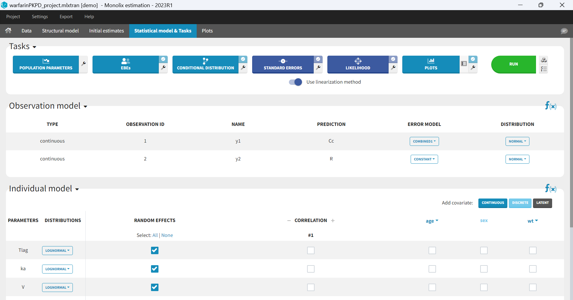
4.1.Observation (error) model
- Introduction
- Defining the residual error model from the Monolix GUI
- Some basic residual error models
- Residual error models for bounded data
- Autocorrelated residuals
- Using different error models per group/study
Objectives: learn how to use the predefined residual error models.
Projects: warfarinPK_project, bandModel_project, autocorrelation_project, errorGroup_project
Introduction
For continuous data, we are going to consider scalar outcomes (\(y_{ij} \in \mathbb{R}\)) and assume the following general model:
$$y_{ij}=f(t_{ij},\psi_i)+ g(t_{ij},\psi_i,\xi)\varepsilon_{ij}$$
for i from 1 to N, and j from 1 to \(\text{n}_{i}\), where \(\psi_i\) is the parameter vector of the structural model f for individual i. The residual error model is defined by the function g which depends on some additional vector of parameters \(\xi\). The residual errors \((\varepsilon_{ij})\) are standardized Gaussian random variables (mean 0 and standard deviation 1). In this case, it is clear that \(f(t_{ij}, \psi_i)\) and \(g(t_{ij}, \psi_i, \xi)\) are the conditional mean and standard deviation of \(y_{ij}\), i.e.,
$$\mathbb{E}(y_{ij} | \psi_i) = f(t_{ij}, \psi_i)~~\textrm{and}~~\textrm{sd}(y_{ij} | \psi_i)= g(t_{ij}, \psi_i, \xi)$$
Available error models
In Monolix, we only consider the function g to be a function of the structural model f, i.e. \(g(t_{ij}, \psi_i, \xi)= g(f(t_{ij}, \psi_i), \xi)\) leading to an expression of the observation model of the form
$$y_{ij}=f(t_{ij},\psi_i)+ g(f(t_{ij}, \psi_i), \xi)\varepsilon_{ij}$$
The following error models are available:
- constant : \(y = f + a \varepsilon\). The function g is constant, and the additional parameter is \(\xi=a\)
- proportional : \(y = f + bf^c \varepsilon\). The function g is proportional to the structural model f, and the additional parameters are \(\xi = (b,c)\). By default, the parameter c is fixed at 1 and the additional parameter is
.
- combined1 : \(y = f + (a+ bf^c) \varepsilon\). The function g is a linear combination of a constant term and a term proportional to the structural model f, and the additional parameters are \(\xi = (a, b)\) (by default, the parameter c is fixed at 1).
- combined2 : \(y = f + \sqrt{a^2+ b^2(f^c)^2} \varepsilon\). The function g is a combination of a constant term and a term proportional to the structural model f (g = bf^c), and the additional parameters are \(\xi = (a, b)\) (by default, the parameter c is fixed at 1).
 .
.Notice that the parameter c is fixed to 1 by default. However, it can be unfixed and estimated.
The assumption that the distribution of any observation \(y_{ij}\) is symmetrical around its predicted value is a very strong one. If this assumption does not hold, we may want to transform the data to make it more symmetric around its (transformed) predicted value. In other cases, constraints on the values that observations can take may also lead us to transform the data.
Available transformations
The model can be extended to include a transformation of the data:
$$u(y_{ij})=u(f(t_{ij},\psi_i)) + g(u(f(t_{ij},\psi_i)) ,\xi) $$
As we can see, both the data \(y_{ij}\) and the structural model f are transformed by the function u so that \(f(t_{ij}, \psi_i)\) remains the prediction of \(y_{ij}\). Classical distributions are proposed as transformation:
- normal: u(y) = y. This is equivalent to no transformation.
- lognormal: u(y) = log(y). Thus, for a combined error model for example, the corresponding observation model writes \(\log(y) = \log(f) + (a + b\log(f)) \varepsilon\). It assumes that all observations are strictly positive. Otherwise, an error message is thrown. In case of censored data with a limit, the limit has to be strictly positive too.
- logitnormal: u(y) = log(y/(1-y)). Thus, for a combined error model for example, the corresponding observation model writes \(\log(y/(1-y)) = \log(f/(1-f)) + (a + b\log(f/(1-f)))\varepsilon\). It assumes that all observations are strictly between 0 and 1. It is also possible to modify these bounds and not “impose” them to be 0 and 1, i.e. to define the logit function between a minimum and a maximum: the function u becomes u(y) = log((y-y_min)/(y_max-y)). Again, in case of censored data with a limit, the limits too must belong strictly to the defined interval.
Any interrogation on what is the formula behind your observation model? There is a button FORMULA on the interface as on the figure below where the observation model is described linking the observation (named CONC in that case) and the prediction (named Cc in that case). Note that \(\epsilon\) is noted e here.
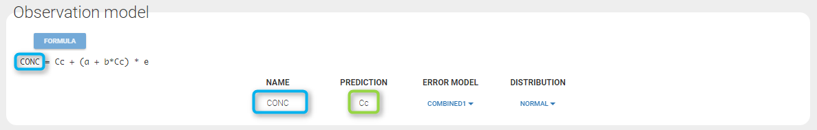
Remarks: In previous Monolix version, only the error was available. Thus, what happens to the errors that are not proposed anymore? Is it possible to have “exponential”, “logit”, “band(0,10)”, and “band(0,100)”? Yes, in this version, we choose to split the observation model between its error model and its distribution. The purpose is to have a more unified vision of models and increase the number of possibilities. Thus, here is how to configure new projects with the previous error model definition.
- “exponential” is an observation model with a constant error model and a lognormal distribution.
- “logit” is an observation model with a constant error model and a logitnormal distribution.
- “band(0,10)” is an observation model with a constant error model and a logitnormal distribution with min and max at 0 and 10 respectively.
- “band(0,100)” is an observation model with a constant error model and a logitnormal distribution with min and max at 0 and 100 respectively.
Defining the residual error model from the Monolix GUI
A menu in the frame Statistical model|Tasks of the main GUI allows one to select both the error model and the distribution as on the following figure (in green and blue respectively)
A summary of the statistical model which includes the residual error model can be displayed by clicking on the button formula.
Some basic residual error models
- warfarinPKlibrary_project (data = ‘warfarin_data.txt’, model = ‘lib:oral1_1cpt_TlagkaVCl.txt’)
The residual error model used with this project for fitting the PK of warfarin is a combined error model, i.e. \(y_{ij} = f(t_{ij}, \psi_i))+ (a+bf(t_{ij}, \psi_i)))\varepsilon_{ij}\) Several diagnosis plots can then be used for evaluating the error model. The observation versus prediction figure below seems ok.
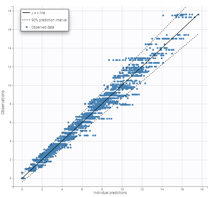
Remarks:
- Figures showing the shape of the prediction interval for each observation model available in Monolix are displayed here.
- When the residual error model is defined in the GUI, a bloc DEFINITION: is then automatically added to the project file in the section [LONGITUDINAL] of <MODEL> when the project is saved:
DEFINITION:
y1 = {distribution=normal, prediction=Cc, errorModel=combined1(a,b)}
Residual error models for bounded data
- bandModel_project (data = ‘bandModel_data.txt’, model = ‘lib:immed_Emax_null.txt’)
In this example, data are known to take their values between 0 and 100. We can use a constant error model and a logitnormal for the transformation with bounds (0,100) if we want to take this constraint into account.
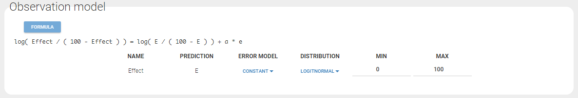
In the Observation versus prediction plot, one can see that the error is smaller when the observations are close to 0 and 100 which is normal. To see the relevance of the predictions, one can look at the 90% prediction interval. Using a logitnormal distribution, we have a very different shape of this prediction interval to take that specificity into account.
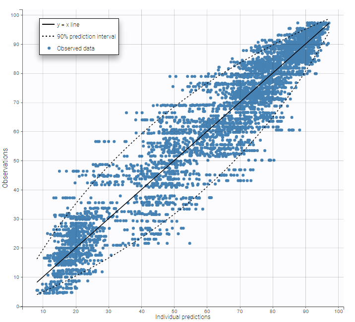
VPCs obtained with this error model do not show any mispecification
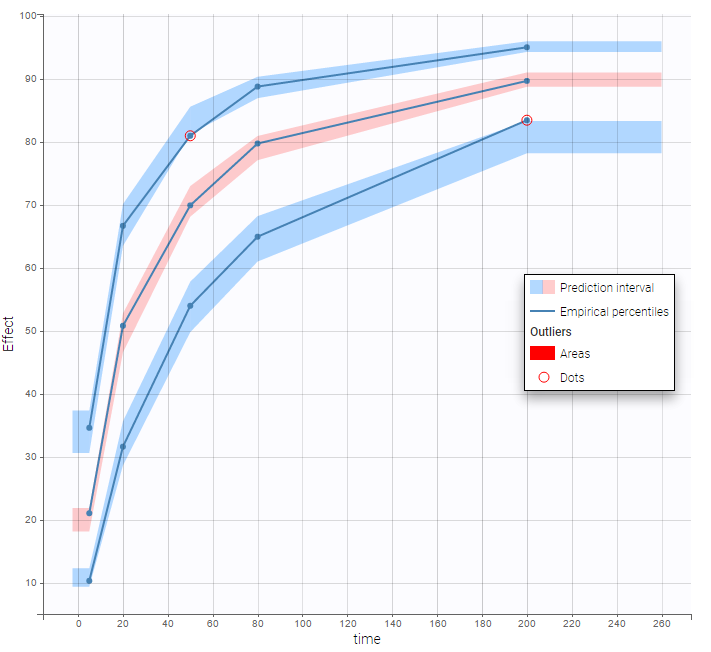 This residual error model is implemented in
 Mlxtran as follows:
DEFINITION:
effect = {distribution=logitnormal, min=0, max=100, prediction=E, errorModel=constant(a)}
Autocorrelated residuals
For any subject i, the residual errors \((\varepsilon_{ij},1 \leq j \leq n_i)\) are usually assumed to be independent random variables. The extension to autocorrelated errors is possible by assuming, that \((\varepsilon_{ij})\) is a stationary autoregressive process of order 1, AR(1), which autocorrelation decreases exponentially:
$$ \textrm{corr}(\varepsilon_{ij},\varepsilon_{i,{j+1}}) = r_i^{(t_{i,j+1}-t_{ij})}$$
where \(0 \leq r_i \leq 1\) for each individual i. If \(t_{ij}=j\) for any (i,j), then \(t_{i,j+1}-t_{i,j}=1\) and the autocorrelation function \(\gamma_i\)for individual i is given by
$$\gamma_i(\tau) = \textrm{corr}(\varepsilon_{ij}, \varepsilon_{i,j+\tau}) = r_i^{\tau}$$
The residual errors are uncorrelated when \(r_i=0\).
- autocorrelation_project (data = ‘autocorrelation_data.txt’, model = ‘lib:infusion_1cpt_Vk.txt’)
Autocorrelation is estimated since the checkbox r is ticked in this project: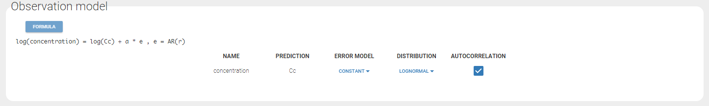 Estimated population parameters now include the autocorrelation r:
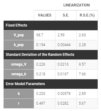 Important remarks:
Monolixaccepts both regular and irregular time grids.- For a proper estimationg of the autocorrelation structure of the residual errors, rich data is required (i.e. a large number of time points per individual) .
- To add autocorrelation, the user should either use the connectors, or write it directly in the Mlxtran
- add “autoCorrCoef=r” in definition “DV = {distribution=normal, prediction=Cc, errorModel=proportional(b), autoCorrCoef=r}” for example
- add “r” as an input parameter.
Using different error models per group/study
- errorGroup_project (data = ‘errorGroup_data.txt’, model = ‘errorGroup_model.txt’)
Data comes from 3 different studies in this example. We want to have the same structural model but use different error models for the 3 studies. A solution consists in defining the column STUDY with the reserved keyword OBSERVATION ID. It will then be possible to define one error model per outcome: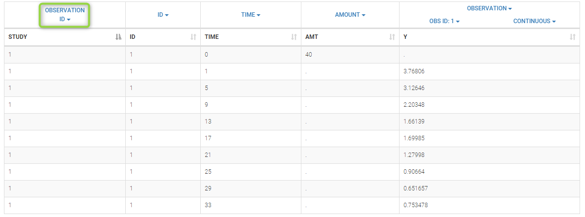
Here, we use the same PK model for the 3 studies:
[LONGITUDINAL]
input = {V, k}

PK:
Cc1 = pkmodel(V, k)
Cc2 = Cc1
Cc3 = Cc1

OUTPUT:
output = {Cc1, Cc2, Cc3}
Since 3 outputs are defined in the structural model, one can now define 3 error models in the GUI:
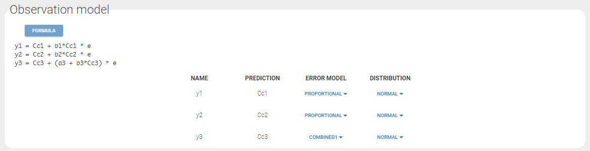 Different residual error parameters are estimated for the 3 studies. One can remark than, even if 2 proportional error models are used for the 2 first studies, different parameters b1 and b2 are estimated:
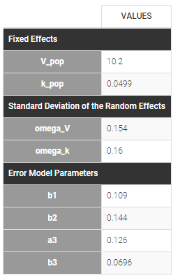
4.2.Individual model
4.2.1.Model for the individual parameters: introduction
What is the individual model and where is it defined in Monolix?
The population approach considers that parameters of the structural model can have a different value for each individual, and the way these values are distributed over individuals and impacted by covariate values is defined in the individual model. The individual model is defined in the lower part of the statistical model tab. This model includes
- distributions for the individual parameters
- which parameters have inter-individual variability (random effects)
- correlation structure of the random effects
- covariate effects on the individual parameters
Theory for the individual model
A model for observations depends on a vector of individual parameters \(\psi_i\). As we want to work with a population approach, we now suppose that \(\psi_i\) comes from some probability distribution \(p_{{\psi_i}}\).
In this section, we are interested in the implementation of individual parameter distributions \((p_{{\psi_i}}, 1\leq i \leq N)\). Generally speaking, we assume that individuals are independent. This means that in the following analysis, it is sufficient to take a closer look at the distribution \(p_{{\psi_i}}\) of a unique individual i. The distribution \(p_{{\psi_i}}\) plays a fundamental role since it describes the inter-individual variability of the individual parameter \(\psi_i\). In Monolix, we consider that some transformation of the individual parameters is normally distributed and is a linear function of the covariates:
\(h(\psi_i) = h(\psi_{\rm pop})+ \beta \cdot ({c}_i – {c}_{\rm pop}) + \eta_i \,, \quad \eta_i \sim {\cal N}(0,\Omega).\)
This model gives a clear and easily interpreted decomposition of the variability of \(h(\psi_i)\) around \(h(\psi_{\rm pop})\), i.e., of \(\psi_i\) around \(\psi_{\rm pop}\):
The component \(\beta \cdot ({c}_i – {c}_{\rm pop})\) describes part of this variability by way of covariates \({c}_i\) that fluctuate around a typical value \({c}_{\rm pop}\).
The random component \(\eta_i\) describes the remaining variability, i.e., variability between subjects that have the same covariate values. By definition, a mixed effects model combines these two components: fixed and random effects. In linear covariate models, these two effects combine. In the present context, the vector of population parameters to estimate is \(\theta = (\psi_{\rm pop},\beta,\Omega)\). Several extensions of this basic model are possible:
We can suppose for instance that the individual parameters of a given individual can fluctuate over time. Assuming that the parameter values remain constant over some periods of time called occasions, the model needs to be able to describe the inter-occasion variability (IOV) of the individual parameters.
If we assume that the population consists of several homogeneous subpopulations, a straightforward extension of mixed effects models is a finite mixture of mixed effects models, assuming for instance that the distribution \(p_{{\psi_i}}\) is a mixture of distributions.
4.2.2.Probability distribution of the individual parameters
- Introduction
- Marginal distributions of the individual parameters
- Correlation structure of the random effects
- Parameters without random effects
- Custom parameter distribution
Objectives: learn how to define the probability distribution and the correlation structure of the individual parameters.
Projects: warfarin_distribution1_project, warfarin_distribution2_project, warfarin_distribution3_project, warfarin_distribution4_project
Introduction
One way to extend the use of Gaussian distributions is to consider that some transformation of the parameters in which we are interested is Gaussian, i.e., assume the existence of a monotonic function \(h\) such that \(h(\psi)\) is normally distributed. Then, there exists some \(\omega\) such that, for each individual i:
\(h(\psi_i) \sim {\cal N}(h(\bar{\psi}_i), \omega^2)\)
where \(\bar{\psi}_i\) is the predicted value of \(\psi_i\). In this section, we consider models for the individual parameters without any covariate. Then, the predicted value of \(\psi_i\) is the \(\bar{\psi}_i = \psi_{\rm pop}\) and
\(h(\psi_i) \sim {\cal N}(h(\psi_{pop}), \omega^2)\)
The transformation \(h\) defines the distribution of \(\psi_i\). Some predefined distributions/transformations are available in Monolix:
- Normal distribution in ]-inf,+inf[:
In that case, \(h(\psi_i) = \psi_i\).
Note: the two mathematical representations for normal distributions are equivalent:
\( \psi_i \sim {\cal N}(\bar{\psi}_{i}, \omega^2) ~~\Leftrightarrow~~ \psi_i = \bar{\psi}_i + \eta_i, ~~\text{where}~~\eta_i \sim {\cal N}(0,\omega^2).\)
- Log-normal distribution in ]0,+inf[:
In that case, \(h(\psi_i) = log(\psi_i)\). A log-normally random variable takes positive values only. A log-normal distribution looks like a normal distribution for a small variance \(\omega^2\). On the other hand, the asymmetry of the distribution increases when \(\omega^2\) increases.
Note: the two mathematical representations for log-normal distributions are equivalent:
\(\log(\psi_i) \sim {\cal N}(\log(\bar{\psi}_{i}), \omega^2) ~~\Leftrightarrow~~ \log(\psi_i)=\log(\bar{\psi}_{i})+\eta_i~~\Leftrightarrow~~ \psi_i = \bar{\psi}_i e^{\eta_i}, ~~\text{where}~~\eta_i \sim {\cal N}(0,\omega^2).\)
\(\bar{\psi}_i\) represents the typical value (fixed effect) and \(\omega\) the standard deviation of the random effects, which is interpreted as the inter-individual variability. Note that \(\bar{\psi}_i\) is the median of the distribution (neither the mean, nor the mode).
- Logit-normal distribution in ]0,1[:
In that case, \(h(\psi_i) = log\left(\frac{\psi_i}{1-\psi_i}\right)\). A random variable \(\psi_i\) with a logit-normal distribution takes its values in ]0,1[. The logit of \(\psi_i\) is normally distributed, i.e.,
\(\text{logit}(\psi_i) = \log \left(\frac{\psi_i}{1-\psi_i}\right) \ \sim \ \ {\cal N}( \text{logit}(\bar{\psi}_i), \omega^2) ~~\Leftrightarrow~~ \text{logit}(\psi_i) = \text{logit}(\bar{\psi}_i) + \eta_i, ~~\text{where}~~\eta_i \sim {\cal N}(0,\omega^2)\)
Note that:
\( m = \text{logit}(\psi_i) = \log \left(\frac{\psi_i}{1-\psi_i}\right) ~~\Leftrightarrow~~ \psi_i = \frac{\exp(m)}{1+\exp(m)} \)
- Generalized logit-normal distribution in ]a,b[:
In that case, \(h(\psi_i) = log\left(\frac{\psi_i – a}{b-\psi_i}\right)\). A random variable \(\psi_i\) with a logit-normal distribution takes its values in ]a,b[. The logit of \(\psi_i\) is normally distributed, i.e.,
\(\text{logit}_{(a,b)}(\psi_i) = \log \left(\frac{\psi_i – a}{b-\psi_i}\right) \ \sim \ \ {\cal N}( \text{logit}_{(a,b)}(\bar{\psi}_i), \omega^2) ~~\Leftrightarrow~~ \text{logit}_{(a,b)}(\psi_i) = \text{logit}_{(a,b)}(\bar{\psi}_i) + \eta_i, ~~\text{where}~~\eta_i \sim {\cal N}(0,\omega^2)\)
Note that:
\( m = \text{logit}_{(a,b)}(\psi_i) = \log \left(\frac{\psi_i – a}{b-\psi_i}\right) ~~\Leftrightarrow~~ \psi_i = \frac{b \exp(m)+a}{1+\exp(m)} \)
- Probit-normal distribution:
The probit function is the inverse cumulative distribution function (quantile function) \(\Phi^{-1}\) associated with the standard normal distribution \({\cal N}(0,1)\). A random variable \(\psi\) with a probit-normal distribution also takes its values in ]0,1[.
\(\text{probit}(\psi_i) = \Phi^{-1}(\psi_i) \ \sim \ {\cal N}( \Phi^{-1}(\bar{\psi}_i), \omega^2) .\)
To chose one of these distribution in the GUI, click on the distribution corresponding to the parameter you want to change in the individual model part and choose the corresponding distribution.

Remarks:
- If you change your distribution and your population parameter is not valid, then an error message is thrown. Typically, when you want to change your distribution to a log normal distribution, make sure the associated population parameter is strictly positive.
- When creating a project, the default proposed distribution is lognormal.
- Logit transformations can be generalized to any interval (a,b) by setting \( \psi_{(a,b)} = a + (b-a)\psi_{(0,1)}\) where \(\psi_{(0,1)}\) is a random variable that takes values in (0,1) with a logit-normal distribution. Thus, if you need to have bounds between a and b, you need to modify your structural model to reshape a parameter between 0 and 1 and use a logit or a probit distribution. Examples are shown on this page.
- “Adapted” Logit-normal distribution:
Another interesting possibility is to “extend” the logit distribution to be bounded in [a, b] rather than in [0, 1]. It is possible starting from the 2019 version. For that, set your parameter in a logit normal distribution. The setting button appear next to the distribution.
Clicking on it will allow to define your bounds as in the following figure.
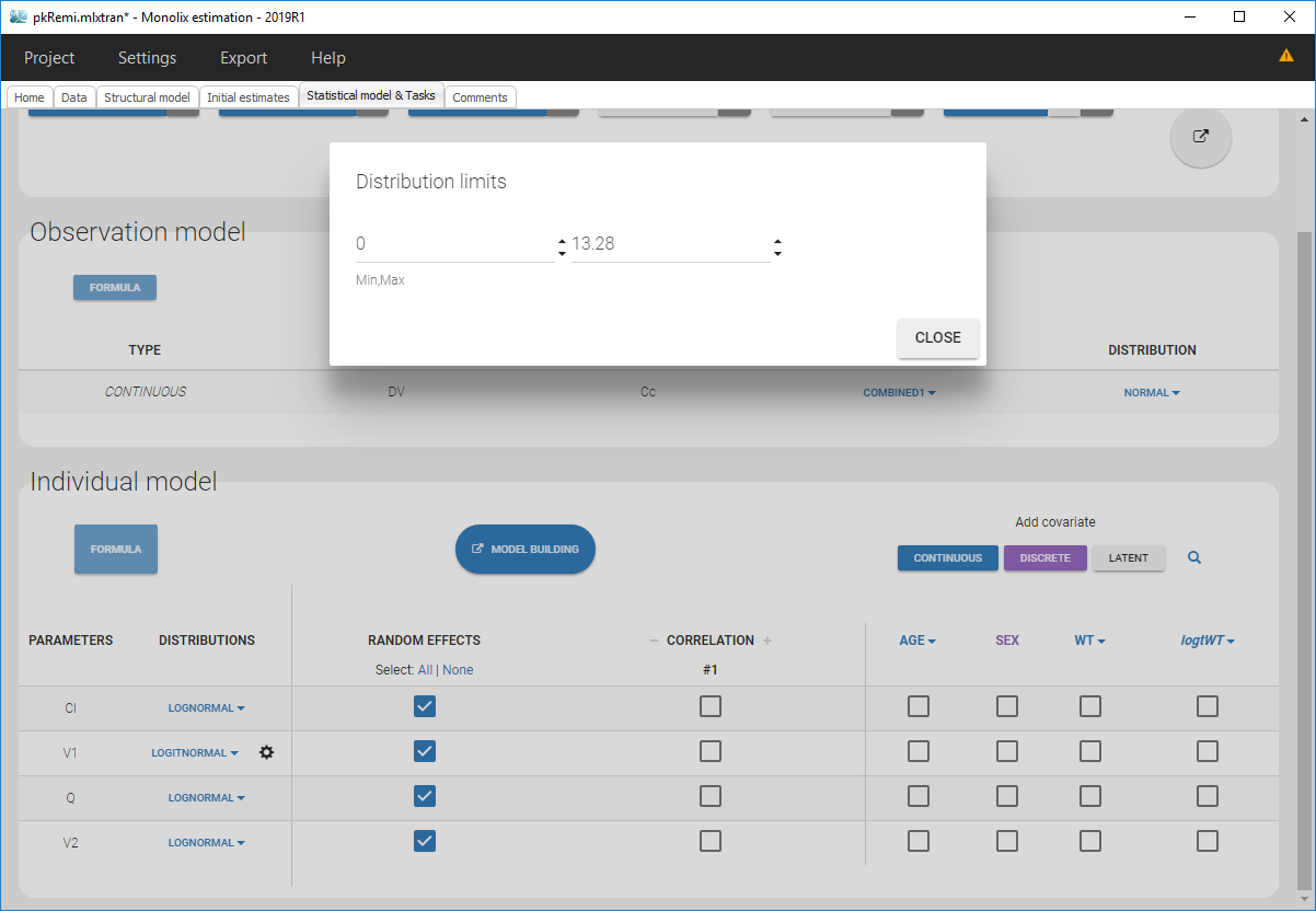
Notice that if your parameter initial value is not in [0, 1], the bounds are automatically adapted and the following warning message is proposed “The initial value of XX is greater than 1: the logit limit is adjusted”
Marginal distributions of the individual parameters
- warfarin_distribution1_project (data = ‘warfarin_data.txt’, model = ‘lib:oral1_1cpt_TlagkaVCl.txt’)
We use the warfarin PK example here. The four PK parameters Tlag, ka, V and Cl are log-normally distributed. LOGNORMAL distribution is then used for these four log-normal distributions in the main Monolix graphical user interface:

The distribution of the 4 PK parameters defined in the MonolixGUI is automatically translated into Mlxtran in the project file:
[INDIVIDUAL]
input = {Tlag_pop, omega_Tlag, ka_pop, omega_ka, V_pop, omega_V, Cl_pop, omega_Cl}
DEFINITION:
Tlag = {distribution=lognormal, typical=Tlag_pop, sd=omega_Tlag}
ka = {distribution=lognormal, typical=ka_pop, sd=omega_ka}
V = {distribution=lognormal, typical=V_pop, sd=omega_V}
Cl = {distribution=lognormal, typical=Cl_pop, sd=omega_Cl}
Estimated parameters are the parameters of the 4 log-normal distributions and the parameters of the residual error model:
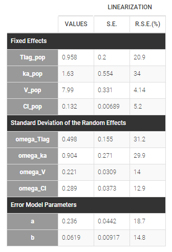
Here, \(V_{\rm pop} = 7.94\) and \(\omega_V=0.326\) means that the estimated population distribution for the volume is: \(\log(V_i) \sim {\cal N}(\log(7.94) , 0.326^2)\) or, equivalently, \(V_i = 7.94 e^{\eta_i}\) where \(\eta_i \sim {\cal N}(0,0.326^2)\).
Remarks:
- \(V_{\rm pop} = 7.94\) is not the population mean of the distribution of \(V_i\), but the median of this distribution (in that case, the mean value is 7.985). The four probability distribution functions are displayed figure
Parameter distributions:
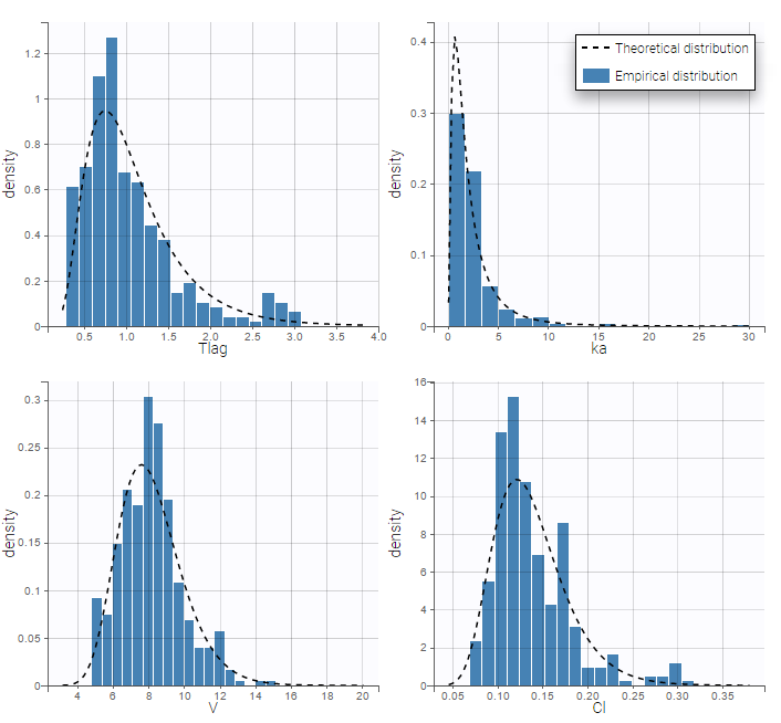
- \(V_{\rm pop}\) is not the population mean of the distribution of \(V_i\), but the median of this distribution. The same property holds for the 3 other distributions which are not Gaussian.
- Here, standard deviations \(\omega_{Tlag}\), \(\omega_{ka}\), \(\omega_V\) and \(\omega_{Cl}\) are approximately the coefficients of variation (CV) of Tlag, ka, V and Cl since these 4 parameters are log-normally distributed with variances < 1.
- warfarin_distribution2_project (data = ‘warfarin_data.txt’, model = ‘lib:oral1_1cpt_TlagkaVCl.txt’)
Other distributions for the PK parameters are used in this project:
- NORMAL for Tlag, we fix the population value \(Tlag_{\text{pop}}\) to 1.5 and the standard deviation \(\omega_{\rm Tlag}\) to 1:
- NORMAL for ka,
- NORMAL for V,
- and LOGNORMAL for Cl
Estimated parameters are the parameters of the 4 transformed normal distributions and the parameters of the residual error model:
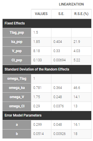
Here, \( Tlag_{\rm pop} = 1.5\) and \(\omega_{Tlag}=1\) means that \(Tlag_i \sim {\cal N}(1.5, 1^2)\) while \(Cl_{\rm pop} = .133\) and \(\omega_{Cl}=..29\) means that \(log(Cl_i) \sim {\cal N}(log(.133), .29^2)\). The four probability distribution functions are displayed Figure Parameter distributions:
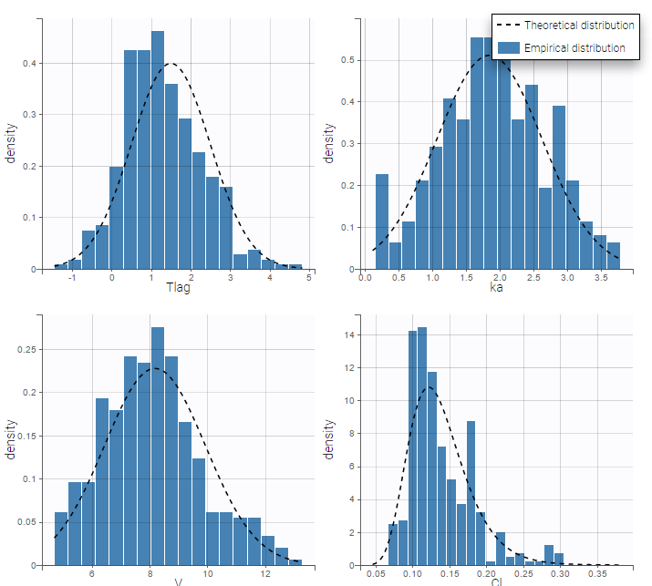
Correlation structure of the random effects
Dependency can be introduced between individual parameters by supposing that the random effects \(\eta_i\) are not independent. This means considering them to be linearly correlated.
- warfarin_distribution3_project (data = ‘warfarin_data.txt’, model = ‘lib:oral1_1cpt_TlagkaVCl.txt’)
Defining correlation between random effects in the interface
To introduce correlations between random effects in Monolix, one can define correlation groups. For example, two correlation groups are defined on the interface below, between \(\eta_{V,i}\) and \(\eta_{Cl,i}\) (#1 in that case) and between \(\eta_{Tlag,i}\) and \(\eta_{ka,i}\) in an other group (#2 in that case):

To define a correlation between the random effects of V and Cl, you just have to click on the check boxes of the correlation for those two parameters. If you want to define a correlation between the random effects ka and Tlag independently of the first correlation group, click on the + next to CORRELATION to define a second group and click on the check boxes corresponding to the parameters ka and Tlag under the correlation group #2. Notice, that as the random effects of Cl and V are already in the correlation group #1, these random effects can not be used in another correlation group. When three of more parameters are included in a correlation groups, all pairwise correlations will be estimated. It is not instance not possible to estimate the correlation between \(\eta_{ka,i}\) and \(\eta_{V,i}\) and between \(\eta_{Cl,i}\) and \(\eta_{V,i}\) but not between \(\eta_{Cl,i}\) and \(\eta_{ka,i}\).
It is important to mention that the estimated correlations are not the correlation between the individual parameters (between \(Tlag_i\) and \(ka_i\), and between \(V_i\) and \(Cl_i\)) but the (linear) correlation between the random effects (between \(\eta_{Tlag,i}\) and \(\eta_{ka,i}\), and between \(\eta_{V,i}\) and \(\eta_{Cl,i}\) respectively).
Remarks
- If the box is greyed, it means that the associated random effects can not be used in a correlation group, as in the following cases
- when the parameter has no random effects
- when the random effect of the parameter is already used in another correlation group
- There are no limitation in terms of number of parameters in a correlation group
- You can have a look in the FORMULA to have a recap of all correlations
- In case of inter-occasion variability, you can define the correlation group for each level of variability independently.
- The initial value for the correlations is zero and cannot be changed.
- The correlation value cannot be fixed.
Estimated population parameters now include these 2 correlations:
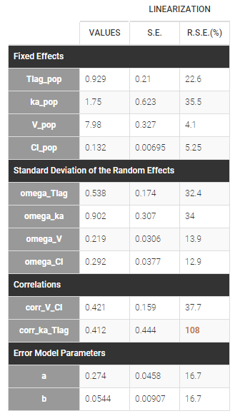
Notice that the high uncertainty on \(\text{corr_ka_Tlag}\) suggests that the correlation between \(\eta_{Tlag,i}\) and \(\eta_{ka,i}\) is not reliable.
How to decide to include correlations between random effects?
The scatterplots of the random effects can hint at correlations to include in the model. This plot represents the joint empirical distributions of each pair of random effects. The regression line (in pink below) and the correlation coefficient (“information” toggle in the settings) permits to visually detect tendencies. If “conditional distribution” (default) is chosen in the display settings, the displayed random effects are calculated using individual parameters sampled from the conditional distribution, which permits to avoid spurious correlations (see the page on shrinkage for more details). If a large correlation is present between a pair of random effects, this correlation can be added to the model in order to be estimated as a population parameter.
Depending on a number of random effects values used to calculate the correlation coefficient, a same correlation value can be more or less significant. To help the user identify significant correlations, Pearson’s correlation tests are performed in the “Result” tab, “Tests” section. If no significant correlation is found, like for the pair \(\eta_{Tlag}\) and \(\eta_{Cl}\) below, the distributions can be assumed to be independent. However, if a significant correlation appears, like for the pair \(\eta_V\) and \(\eta_{Cl}\) below, it can be hypothesized that the distributions are not independent and that the correlation must be included in the model and estimated. Once the correlation is included in the model, the random effects for \(V\) and \(Cl\) are drawn from the joint distribution rather than from two independent distributions.
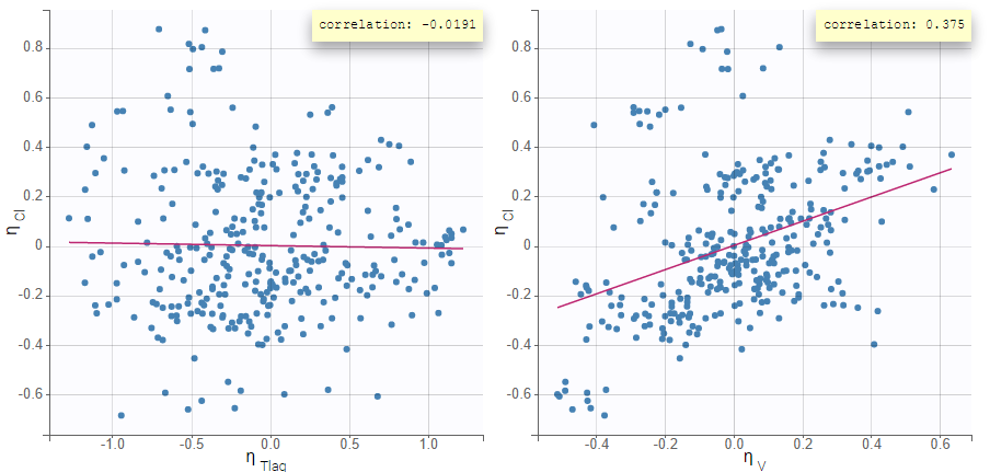 |
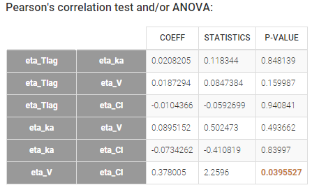 |
How do the correlations between random effects affect the individual model?
In this example the model has four parameters Tlag, ka, V and Cl. Without correlation, the individual model is:
\(log(Tlag) = log(Tlag_{pop}) + \eta_{Tlag}\)
\(log(ka) = log(ka_{pop}) + \eta_{ka}\)
\(log(V) = log(V_{pop}) + \eta_V\)
\(log(Cl) = log(Cl_{pop}) + \eta_{Cl}\)
The random effects follow normal distributions: \((\eta_{Tlag,i},\eta_{ka,i},\eta_{V,i},\eta_{Cl,i}) \sim \mathcal{N}(0,\Omega)\)
\(\Omega\) is the variance-covariance matrix defining the distributions of the vectors of random effects, here:
\(\Omega = \begin{pmatrix} \omega_{Tlag}^2 & 0 & 0 & 0 \\ 0 & \omega_{ka}^2 & 0 & 0 \\ 0 & 0 & \omega_V^2 & 0 \\ 0 & 0 & 0 & \omega_{Cl}^2 \end{pmatrix}\)
In this example, two correlations between \(\eta_{Tlag}\) and \(\eta_{ka}\) and between \(\eta_{V}\) and \(\eta_{Cl}\) are added to the model. They are defined with two population parameters called \(\text{corr_Tlag_ka}\) and \(\text{corr_V_Cl}\) that appear in the variance-covariance matrix. So the only difference in the individual model is in \(\Omega\), that is now:
\(\Omega = \begin{pmatrix} \omega_{Tlag}^2 & \omega_{Tlag} \omega_{ka} \text{corr_Tlag_ka} & 0 & 0 \\ \omega_{Tlag} \omega_{ka} \text{corr_Tlag_ka} & \omega_{ka}^2 & 0 & 0 \\ 0 & 0 & \omega_V^2 & \omega_{V} \omega_{Cl} \text{corr_V_Cl} \\ 0 & 0 & \omega_{V} \omega_{Cl} \text{corr_V_Cl} & \omega_{Cl}^2 \end{pmatrix}\)
So the correlation matrix is related to the variance-covariance matrix \(\Omega\) as:
$$\text{corr}(\theta_i,\theta_j)=\frac{\text{covar}(\theta_i,\theta_j)}{\sqrt{\text{var}(\theta_i)}\sqrt{\text{var}(\theta_j)}}$$
Why should the correlation be estimated as part of the population parameters?
The effect of correlations is especially important when simulating parameters from the model. This is the case in the VPC or when simulating new individuals in Simulx to assess the outcome of a different dosing scenario for instance. If in reality individuals with a large distribution volume also have a large clearance (i.e there is a positive correlation between the random effects of the volume and the clearance), but this correlation has not been included in the model, then the concentrations predicted by the model for a new cohort of individuals will display a larger variability than they would in reality.
How do the EBEs change after having included correlation in the model?
Before adding correlation in the model, the EBEs or the individual parameters sampled from the conditional distribution may already be correlated, as can be seen in the “correlation between random effects” plot. This is because the individual parameters (EBEs or sampled) are based on the individual conditional distributions, which takes into account the information given by the data. Especially when the data is rich, the data can indicate that individuals with a large volume of distribution also have a large clearance, even if this correlation is not yet included in the model.
Including the correlation in the model as a population parameter to estimate allows to precisely estimate its value. Usually, one can see a stronger correlation for the corresponding pair of random effects when the correlation is included in the model compared to when it is not. In this example, after including the correlations in the individual model, the joint distribution of \(\eta_{V}\) and \(\eta_{Cl}\) displays a higher correlation coefficient (0.439 compared to 0.375 previously):
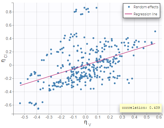
- warfarin_distribution4_project (data = ‘warfarin_data.txt’, model = ‘lib:oral1_1cpt_TlagkaVCl.txt’)
In this example, \(Tlag_i\) does not vary in the population, which means that \(\eta_{Tlag,i}=0\) for all subjects i, while the three other random effects are correlated:

Estimated population parameters now include the 3 correlations between \(\eta_{ka,i}\), \(\eta_{V,i}\) and \(\eta_{Cl,i}\) :
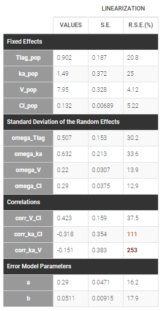
Parameters without random effects
Adding/removing inter-individual variability
By default, all parameters have inter-individual variability. To remove it, click on the checkbox of the random effect column:
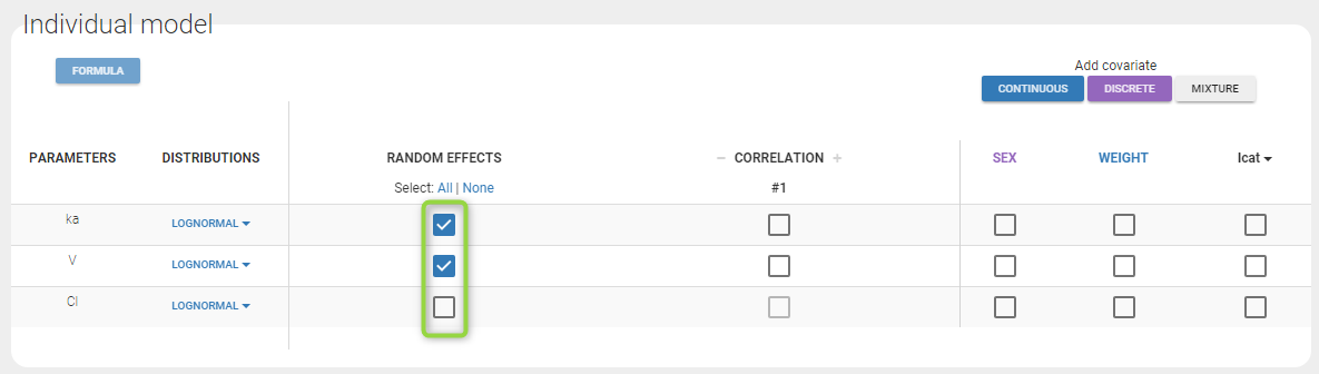
How the parameters with no variability are estimated is explained here.
Custom parameter distributions
Some datasets may require more complex parameter distributions that those pre-implemented in the Monolix GUI. This video shows how to implement a lognormal distribution with Box-Cox transformation and how to bound a parameter between two values using a transformed logit distribution (this latter case can be handled automatically from Monolix2019R1).
4.2.3.Bounded parameter distribution
Bounded parameters in the interface
Starting from the 2019 version, it is possible to “extend” the logit distribution to be bounded in [a, b] rather than in [0, 1]. For that, set your parameter in a logit normal distribution. The setting button appear next to the distribution.
Clicking on it will allow to define your bounds as in the following figure.
Notice that if your parameter initial value is not in [0, 1], the bounds are automatically adapted and the following warning message is proposed “The initial value of XX is greater than 1: the logit limit is adjusted”
Bounded parameters in the structural model
For versions of Monolix below 2019R1, a bounded parameter distribution, for example between a and b, can not be set directly through the interface, but have to be defined in two steps: (1) an auxiliary parameter and its distribution choice in the GUI, and (2) a transformation of the auxiliary parameter into the parameter of interest in the structural model file.
The same approach should be used in Monolix2019R1 to define a single bound (upper or lower).
Let’s take a simple PK example where a volume V is constrained. The structural model for this example is:
[LONGITUDINAL]
input = {V, k}
EQUATION:
; PK model definition
Cc = pkmodel(V, k)
- Thus, to have a parameter V between two bounds a=1 and b=10, you have to define the structural model as below
[LONGITUDINAL]
input = {V_logit, k}
EQUATION:
; PK model definition
a = 1
b = 10
V_bound = a+V_logit*(b-a)
Cc = pkmodel(V=V_bound, k)
In the “Statistical model & Tasks” tab of the GUI, the distribution for V_logit should be set to LOGIT.
- To have a parameter V larger than a=1 (with ‘a’ different from 0), you have to define the structural model as below
[LONGITUDINAL]
input = {V_log, k}
EQUATION:
; PK model definition
a = 1
V_bound = a+V_log
Cc = pkmodel(V=V_bound, k)
In the “Statistical model & Tasks” tab of the GUI, the distribution for V_log should be set to LOGNORMAL.
- To have a parameter V smaller than b=10, you have to define the structural model as below
[LONGITUDINAL]
input = {V_log, k}
EQUATION:
; PK model definition
b = 10
V_bound = b-V_log
Cc = pkmodel(V=V_bound, k)
In the “Statistical model & Tasks” tab of the GUI, the distribution for V_log should be set to LOGNORMAL.
Notice that, using that transformation, you have to multiply the standard error of V_logit by (b-a) in the first case to have the standard error of the initial V_bound parameter. It is not necessary for the two other cases as it is an offset. In addition, you can output V_bound for each individual using the table statement.
4.2.4.Model for individual covariates
- Model with continuous covariates
- Model with categorical covariates
- Transforming categorical covariates
- The same covariate effect for several parameters
- Complex parameter covariate relationships (such as Michaelis-Menten or Hill dependencies, time-dependent covariates, or covariate-dependent standard deviations of random effects)
Objectives: learn how to implement a model for continuous and/or categorical covariates.
Projects: warfarin_covariate1_project, warfarin_covariate2_project, warfarin_covariate3_project, phenobarbital_project
Model with continuous covariates
- warfarin_covariate1_project (data = ‘warfarin_data.txt’, model = ‘lib:oral1_1cpt_TlagkaVCl.txt’)
The warfarin data contains 2 individual covariates: weight which is a continuous covariate and sex which is a categorical covariate with 2 categories (1=Male, 0=Female). We can ignore these columns if are sure not to use them, or declare them using respectively the reserved keywords CONTINUOUS COVARIATE and CATEGORICAL COVARIATE to define continuous and categorical covariate.
Even if these 2 covariates are now available, we can choose to define a model without any covariate by not clicking on any check box in the covariate model.
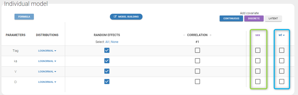
Here, an unchecked box in the line of the parameter V and the column of the covariate wt means that there is no relationship between weight and volume in the model. A diagnosis plot Individual parameters vs covariates is generated which displays possible relationships between covariates and individual parameters (even if these covariates are not used in the model):
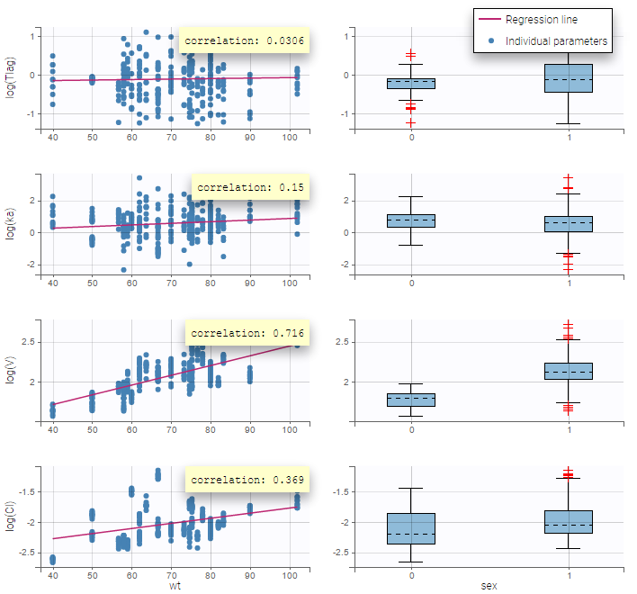
On the figure, we can see a strong correlation between the volume V and both the weight wt and the sex. One can also see a correlation between the clearance and the weight wt. Therefore, the next step is to add some covariate to our model.
- warfarin_covariate2_project (data = ‘warfarin_data.txt’, model = ‘lib:oral1_1cpt_TlagkaVCl.txt’)
We decide to use the weight in this project in order to explain part of the variability of \(V_i\) and \(Cl_i\). We will implement the following model for these two parameters:
$$\log(V_i) = \log(V_{\rm pop}) + \beta_V \log(w_i/70) + \eta_{V,i} ~~\text{and}~~\log(Cl_i) = \log(Cl_{\rm pop}) + \beta_{Cl} \log(w_i/70) + \eta_{Cl,i}$$
which means that population parameters of the PK parameters are defined for a typical individual of the population with weight = 70kg.
More details about the model
The model for \(V_{i}\) and \(Cl_{i}\) can be equivalently written as follows:
$$ V_i = V_{\rm pop} ( w_i/70 )^{\beta_V} e^{ \eta_{V,i} } ~~\text{and}~~ Cl_i = Cl_{\rm pop} ( w_i/70 )^{\beta_{Cl}} e^{ \eta_{Cl,i} }$$
The individual predicted values for \(V_i\) and \(Cl_i\) are therefore
$$\bar{V}_i = V_{\rm pop} \left( w_i/70 \right)^{\beta_V} ~~\text{and}~~ \bar{Cl}_i = Cl_{\rm pop} \left( w_i/70 \right)^{\beta_{Cl}} $$
and the statistical model describes how \(V_i\) and \(Cl_i\) are distributed around these predicted values:
$$ \log(V_i) \sim {\cal N}( \log(\bar{V}_i) , \omega^2_V) ~~\text{and}~~\log(Cl_i) \sim {\cal N}( \log(\bar{Cl}_i) , \omega^2_{Cl}) $$
Here, \(\log(V_i)\) and \(\log(Cl_i)\) are linear functions of \(\log(w_i/70)\): we then need to transform first the original covariate \(w_i\) into \(\log(w_i/70)\) by clicking on the button CONTINUOUS next to ADD COVARIATE (blue button). Then, the following pop up arises
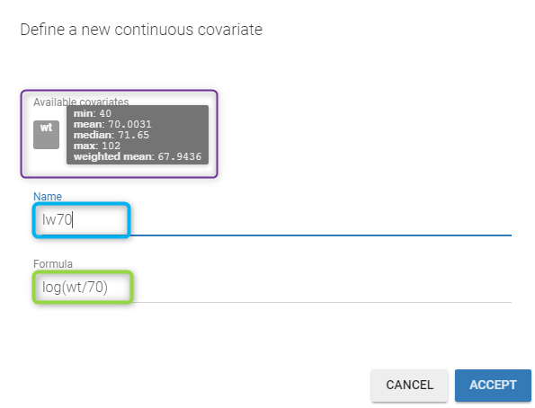
You have to
- define the name of the covariate you want to add (the blue frame).
- define the associated equation (the green frame).
- click on the ACCEPT button
Remarks
- You can define any formula for your covariate as long as you use mathematical functions available in the Mlxtran language.
- You can use any covariate available in the list of covariates proposed in the window. Thus, if you have a Height and Weight as covariates, you can directly compute the Body Mass Index.
- If you go over a covariate with your mouse, all the information (min, mean, median, max and weighted mean) are displayed as a tooltip. The weighted mean is defined as \[ \text{weighted mean} (cov) = \exp \Big( \sum_i \frac{\text{nbObs}_i }{\text{nbObs}} \log(cov_i) \Big)\] where \(\text{nbObs}_i\) is the number of observation for the \(i^{th}\) individual and \(\text{nbObs}\) is the total number of observations.
- If you click on the covariate name, it will be written in the formula.
- You can use this formula box to replace missing continuous covariate values by an imputed value. This is explained in the feature of the week #141 below. For example, if your continuous covariate takes only positive values, you can use a negative value for the missing values in your dataset, for example -99, and enter the following formula: max(COV,0) + min(COV,0)/COV*ImputedValue with the desired ImputedValue (COV is thAse name of your covariate).
We then define a new covariate model, where \(\log(V_i)\) and \(\log(Cl_i)\) are linear functions of the transformed weight \(lw70_i\) as shown on the following figure:

Notice that by clicking on the button FORMULA, you have the display of all the individual model equations. Coefficients \(\beta_{V}\) and \(\beta_{Cl}\) are now estimated with their s.e. and the p-values of the Wald tests are derived to test if these coefficients are different from 0.
Again, a diagnosis plot Individual parameters vs covariates is generated which displays possible relationships between covariates and individual parameters (even if these covariates are not used in the model) as one can see on the figure below on the left. However, as there are covariates on the model, what is interesting is to see if there still are correlation between the random effects and the covariates as one can see on the figure below on the right.
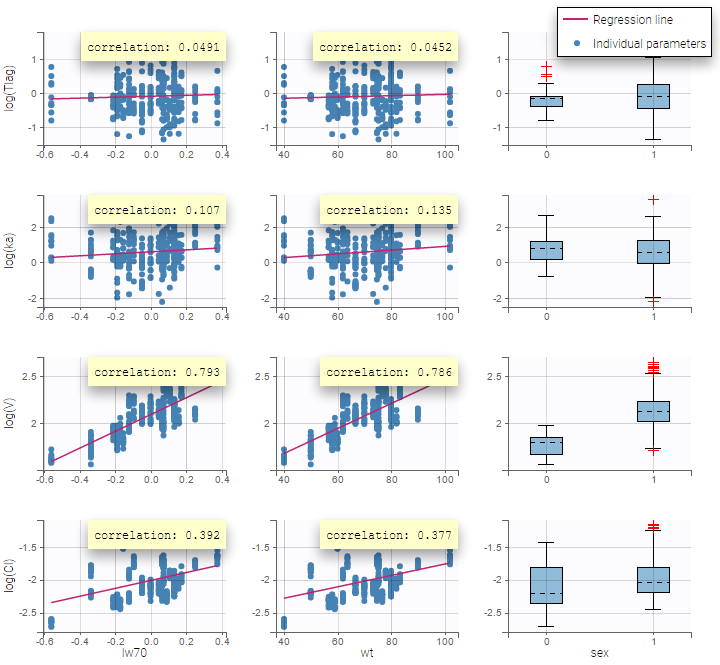 |
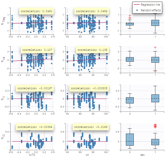 |
|---|
Note: To make it automatically, starting from the 2019 version, there is an arrow next (in purple in the next figure) to the continuous covariate from the data set and propose to add a log transformed covariate centered by the weighted mean.
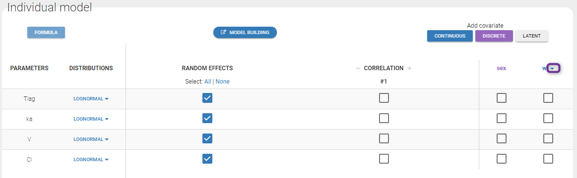
Model with categorical covariates
- warfarin_covariate3_project (data = ‘warfarin_data.txt’, model = ‘lib:oral1_1cpt_TlagkaVCl.txt’)
We use sex instead of weight in this project, assuming different population values of volume and clearance for males and females. More precisely, we consider the following model for \(V_i\) and \(Cl_i\):
$$\log(V_i) = \log(V_{\rm pop}) + \beta_V 1_{sex_i=F} + \eta_{V,i}~~\text{and}~~\log(Cl_i) = \log(Cl_{\rm pop}) + \beta_{Cl} 1_{sex_i=F} + \eta_{Cl,i}$$
where \(1_{sex_i=F} =1\) if individual i is a female and 0 otherwise. Then, \(V_{\rm pop}\) and \(Cl_{\rm pop}\) are the population volume and clearance for males while \(V_{\rm pop}, e^{\beta_V}\) and \(Cl_{\rm pop} e^{\beta_{Cl}}\) are the population volume and clearance for females. By clicking on the purple button DISCRETE, the following window pops up

You have to
- define the name of the covariate you want to add (the blue frame).
- define the associated categories (the green frame).
- click on the ALLOCATE button to define all the categories.
Then, you can
- define the name of the categories (the blue frame).
- define the reference category (the green frame).
- click on ACCEPT
Then, define the covariate model in the main GUI:

Estimated population parameters, including the coefficients \(\beta_V\) and \(\beta_{Cl}\) are displayed with the results:
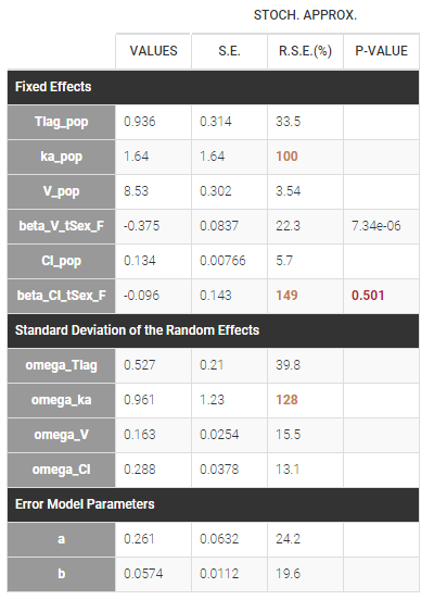 We can display the probability distribution functions of the 4 PK parameters using the
 Individual parameter graphic:
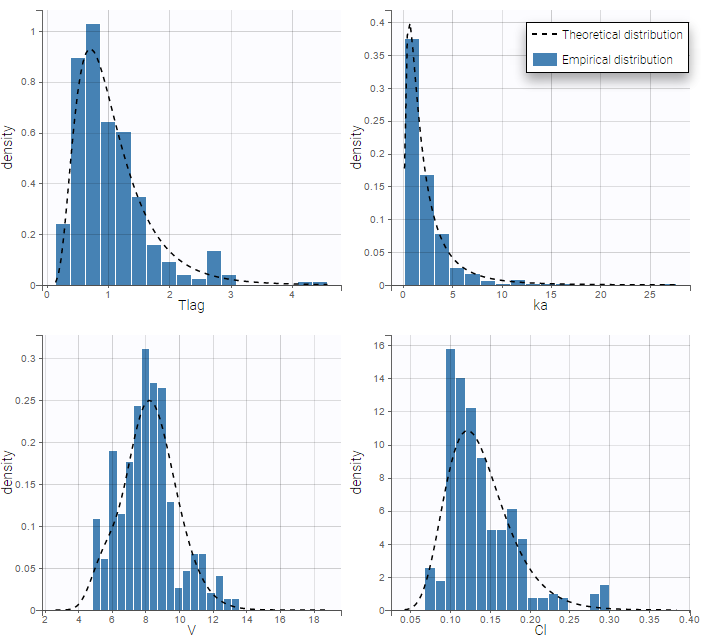
Notice that for the volume and the clearance, the theoretical curve is is not the PDF of a lognormal distribution, due to the impact of the covariate sex.
Calculating the typical value for each category
Cl_pop represents the typical value for the reference category (in the example above SEX=0). The typical value for the other categories can be calculated based on the estimated beta parameters:
- normal distribution: \( Cl_{SEX=1} = Cl_{pop} + beta\_Cl\_SEX\_1 \)
- lognormal distribution: \( Cl_{SEX=1} = Cl_{pop} \times e^{beta\_Cl\_SEX\_1 } \)
- logit distribution: \( F_{SEX=1} = \frac{1}{1+ e^{-\left( \log \left(\frac{F_{pop}}{1-F_{pop}} \right) + beta\_F\_SEX\_1 \right) }} \)
Transforming categorical covariates
- phenobarbital_project (data = ‘phenobarbital_data.txt’, model = ‘lib:bolus_1cpt_Vk.txt’)
The phenobarbital data contains 2 covariates: the weight and the APGAR score which is considered as a categorical covariate. Instead of using the 10 original levels of the APGAR score, we will transform this categorical covariate and create 3 categories: Low = {1,2,3}, Medium = {4, 5, 6, 7} and High={8,9,10}.

If we assume, for instance that the volume is related to the APGAR score, then \(\beta_{V,Low}\) and \(\beta_{V,High}\) are estimated (assuming that Medium is the reference level).
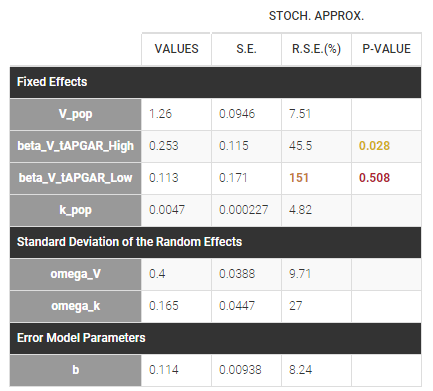
In that case, one can see that both p-values concerning the transformed APGAR covariate are over .05.
The same covariate effect for several parameters
Adding a covariate effect on a parameter in the Individual Model section of the Statistical Model and Tasks tab, creates automatically a corresponding beta parameter (population parameter) that describes the strength of the effect. For example, adding weight WT on a parameter volume V1 creates beta_V1_WT. If you add the same covariate effect on two different parameters, eg. V1 and V2, then Monolix will create two corresponding parameters: beta_V1_WT and beta_V2_WT.
If you need to add the same covariate effect for several parameters, eg. have only one parameter betaWT for both V1 and V2 in the example above, then this covariate effect has to be implemented in the structural model directly. It requires:
-
Reading weight WT from the dataset, so the columnt WT in the dataset has to be tagged as a regressor (not covariate)
-
Defining in the model new volumes with the covariate effect (sample code below, based on a two-compartment model from the PK library)[LONGITUDINAL]input = {WT, betaWT, ka, Cl, V1, Q2, V2}WT = {use=regressor}PK:; Effect of WT on V1, V2V1_withWT = V1*exp(betaWT*WT)V2_withWT = V2*exp(betaWT*WT); Parameter transformationsV = V1_withWTk12 = Q2/V1_withWTk21 = Q2/V2_withWT; PK model definitionCc = pkmodel(ka, V, Cl, k12, k21)OUTPUT:output = {Cc}
-
In the Individual model in the GUI, set normal distribution for “betaWT” – to allow positive and negative values, and remove random effects from it – they are already included in the parameters V1, V2.
4.2.5.Complex parameter-covariate relationships
- Complex parameter-covariate relationships and time-dependent continuous covariates
- Categorical time-varying covariates
- Covariate-dependent parameter
- Covariate-dependent standard deviation
- Transforming a continuous covariate into a categorical covariate
Note that starting from version 2024 on, analytical solutions are used even if a time-varying regressor is used in the model.
Complex parameter-covariate relationships and time-dependent continuous covariates
Covariate-parameter relationships are usually defined via the Monolix GUI, leading for instance to exponential and power law relationships. However more complex parameter-covariate relationships such as Michaelis-Menten or Hill dependencies cannot the defined via the GUI because they cannot be put into the format where the (possibly transformed) covariate is added linearly on the transformed parameter. Similarly, when the covariate value is changing over time and thus not constant for each subject (or each occasion in each subject in case of occasions), the covariate cannot be added to the model via the GUI. In both cases, the effect of the covariate must be tagged as a regressor and the relationship must be defined directly in the model file.
In the following, we will use as an example a Hill relationship between the clearance parameter Cl and the time-varying post-conception age (PCA) covariate, which is a typical way to scale clearance in paediatric pharmacokinetics:
$$Cl_i = Cl_{pop} \frac{PCA^n}{PCA^n+A50^n} e^{\eta_i}$$
where \(Cl_i\) is the parameter value for individual i, \(Cl_{pop}\) the typical clearance for an adult, \(A50\) the PCA for the clearance to reach 50% mature, \(n\) the shape parameter and \(\eta_i\) the random effect for individual i.
Step 1: To make the PCA covariate available as a variable is the model file, the first step is to tag it as a regressor column-type REGRESSOR when loading the data set (instead of using the CONTINUOUS COVARIATE column-type).
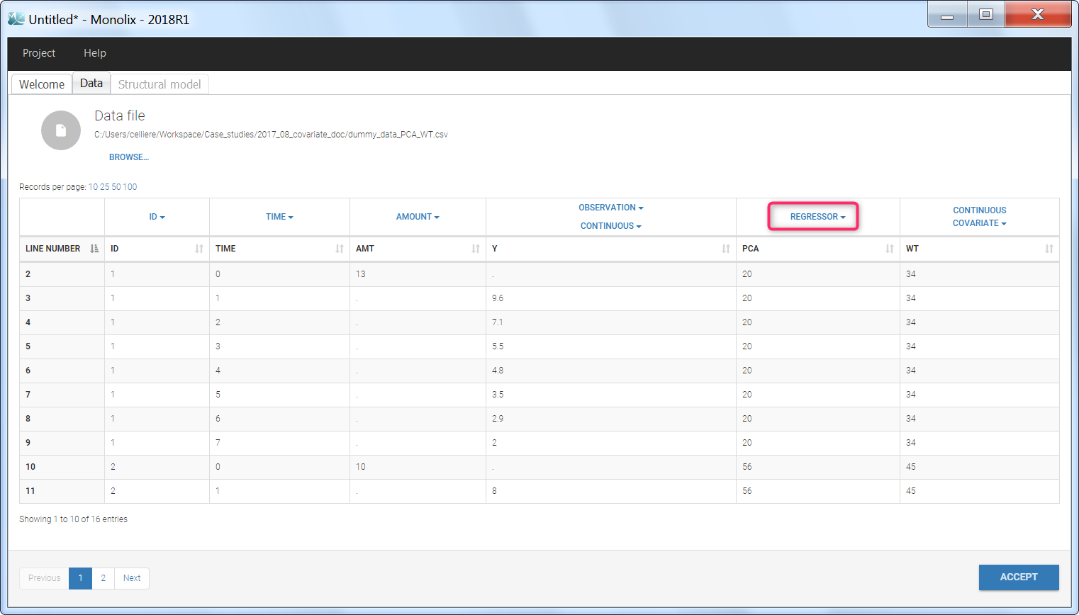
Step 2: In the model file, the PCA covariate is passed as input argument and designated as being a regressor. The clearance Cl, the hill shape parameter n, and the A50 are passed as usual input parameters:
[LONGITUDINAL]
input = {..., Cl, n, A50, PCA, ...}
PCA = {use=regressor}
If several regressors are used, be careful that the regressors are matched by order with the data set columns tagged as REGRESSOR (not by name).
The relationship between the clearance Cl and the post-conception age PCA is defined in the EQUATION: block, before ClwithPCA is used (for instance in a simple (V,Cl) model):
EQUATION:
ClwithPCA = Cl * PCA^n / (PCA^n + A50^n)

Cc = pkmodel(Cl=ClwithPCA, V)
Note that the input parameter Cl includes the random effect ( \(Cl = Cl_{pop} e^{\eta_i} \) ), such that only the covariate term must be added. Because the parameter including the covariate effect CLwithPCA is not a standard keyword for macros, one must write Cl=ClwithPCA.
Step 3: The definition of the parameters in the GUI deserves special attention. Indeed the parameters n and A50 characterize the covariate effect and are the same for all individuals: their inter-individual variability must be removed by unselecting the random effects. On the opposite, the parameter Cl keeps its inter-individual variability, corresponding to the \(e^{\eta_i} \) term.
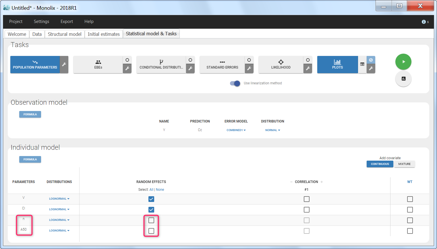
Step 4: When covariates relationships are not defined via the GUI, the p-value corresponding to the Wald test is not automatically outputted. It is however possible to calculate it externally. Assuming that we would like to test if the shape parameter n is significantly different from 1:
$$H_0: \quad \textrm{”}n=1\textrm{”} \quad \textrm{versus} \quad H_1:\quad \textrm{”}n \neq 1\textrm{”}$$
Using the parameter estimate and the s.e outputted by Monolix, we can calculate the Wald statistic:
$$W = \frac{\hat{n}-n_{ref}}{\textrm{s.e}(\hat{n})}$$
with \(\hat{n}\) the estimated value for parameter n, \(n_{ref}\) the reference value for n (here 1) and \(\textrm{s.e}(\hat{n}) \) the standard error for the n estimate.
The test statistic W can then be compared to a standard normal distribution. Below we propose a simple R script to calculate the p-value:
 n_estimated = 1.32
 n_ref = 1
 se_n = 0.12

 W = abs(n_estimated - n_ref)/se_n

 pvalue = 2 * pnorm(W, mean = 0, sd = 1, lower.tail = FALSE)
Note that the factor 2 is added to do a two-sided test.
Categorical time-varying covariates
Categorical covariates may also be time-varying, for instance when the covariate represents concomitant medications over the course of the clinical trial or a fed/fasting state at the time of the dose.
In the following, we will use as an example a concomitant medication categorical covariate with 3 categories: no concomitant drug, concomitant drug 1, and concomitant drug 2. We would like to investigate the effect of the concomitant drug covariate on the clearance Cl.
$$Cl_i = \begin{cases}Cl_{pop} e^{\eta_i} & \textrm{if no concomitant drug} \\ Cl_{pop} (1+\beta_1)e^{\eta_i} & \textrm{if concomitant drug 1} \\ Cl_{pop} (1+\beta_2)e^{\eta_i} & \textrm{if concomitant drug 2} \end{cases}$$
where \(Cl_i\) is the parameter value for individual i, \(Cl_{pop}\) the typical clearance if no concomitant drug, \(\beta_1\) the fractional change in case of concomitant drug 1, \(\beta_2\) the fractional change in case of concomitant drug 2 and \(\eta_i\) the random effect for individual i.
Step 1: Encode the categorical covariate as integers. Indeed, while strings are accepted for the CATEGORICAL COVARIATE column-type, only numbers are accepted for the REGRESSOR column-type. Here we will use 0 = no concomitant medication, 1 = concomitant drug 1 and 2 = concomitant drug 2.
Step 2: To make the COMED covariate available as a variable is the model file, tag it as a column-type REGRESSOR when loading the data set (instead of using the CATEGORICAL COVARIATE column-type).
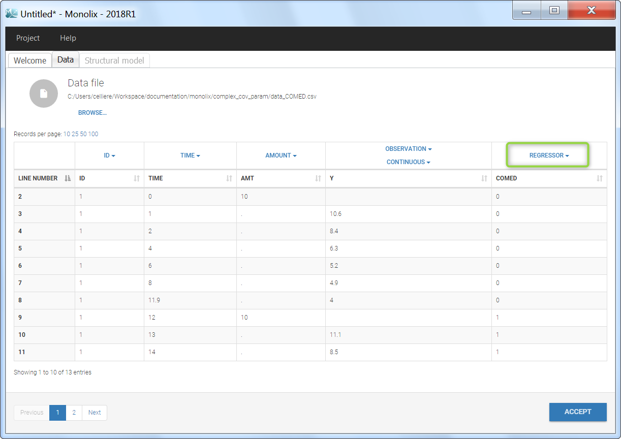
Step 3: In the model file, the COMED covariate is passed as input argument and designated as being a regressor. The clearance Cl, and the two beta parameters are passed as usual input parameters:
[LONGITUDINAL]
input = {..., Cl, beta1, beta2, COMED, ...}
COMED = {use=regressor}
If several regressors are used, be careful that the regressors are matched by order with the data set columns tagged as REGRESSOR (not by name).
To define the COMED covariate impact, we use a if/else statement in the EQUATION: block. The parameter value taking into account the COMED effect (called ClwithCOMED in this example) can then be used in an ODE system or within macros.
EQUATION:
if COMED==0
ClwithCOMED = Cl
elseif COMED==1
ClwithCOMED = Cl * (1+beta1)
else
ClwithCOMED = Cl * (1+beta2)
end

Cc = pkmodel(Cl=ClwithCOMED, V)
Note that the input parameter Cl includes the random effect ( \(Cl = Cl_{pop} e^{\eta_i} \) ), such that only the covariate term must be added. Because the parameter including the covariate effect CLwithCOMED is not a standard keyword for macros, one must write Cl=ClwithCOMED.
If the categorical covariate has only two categories encoded as 0 and 1 (for instance COMED=0 for no concomitant medication and COMED=1 for concomitant medication), it is also possible to write the model in a more compact form:
ClwithCOMED = Cl * (1 + beta * COMED)
Step 4: The definition of the parameters in the GUI deserves special attention. Indeed the parameters beta1 and beta2 characterize the covariate effect and are the same for all individuals: their inter-individual variability must be removed by unselecting the random effects. On the opposite, the parameter Cl keeps its inter-individual variability, corresponding to the \(e^{\eta_i} \) term. In addition, we choose a normal distribution for beta1 and beta2 (with a standard deviation of zero as we have removed the random effects) in order to allow both positive and negative values.
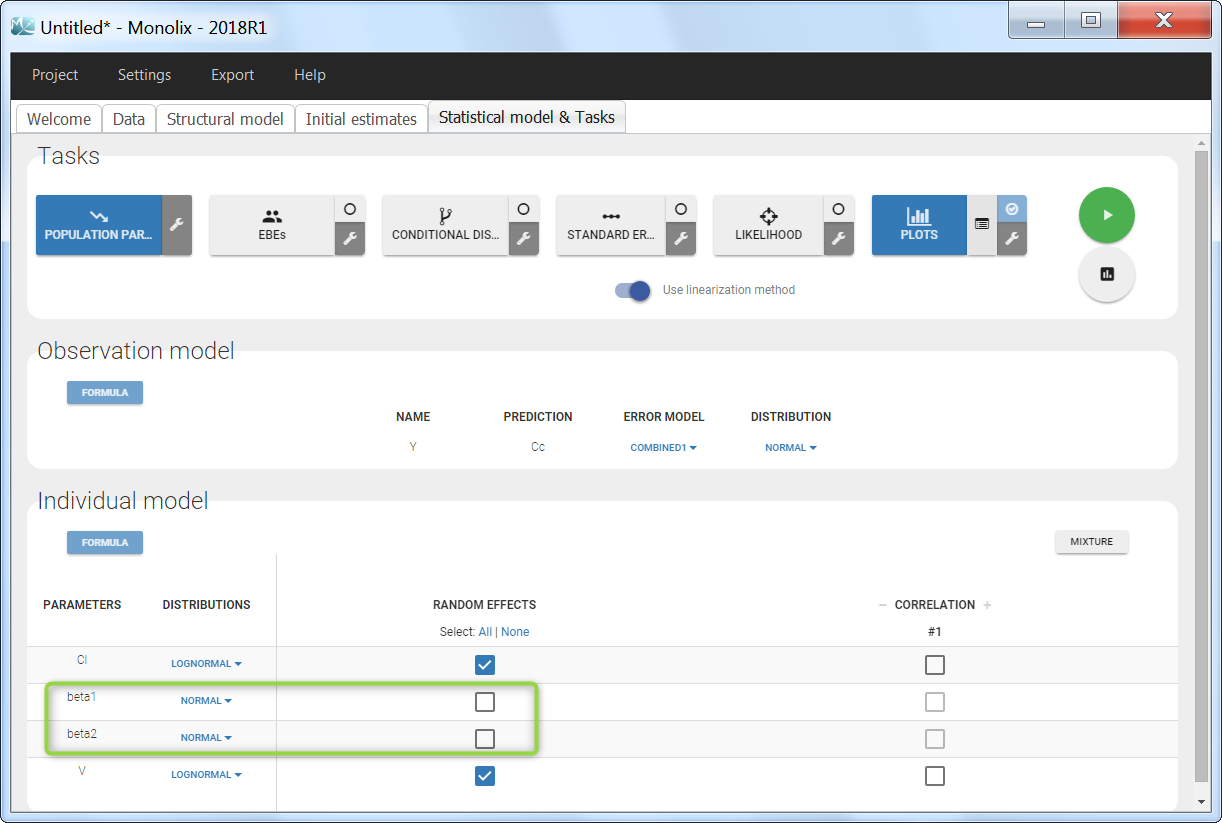
Covariate-dependent parameter
When adding a categorical covariate on a parameter via the GUI, different typical values will be estimated for each group. However, all groups will have the same standard deviation. It can sometimes be useful to consider that the standard deviations also differ between groups. For example, healthy volunteers may have a smaller inter-individual variability than patients.
From the 2018R1 version on, categorical covariates affecting both the typical value and the standard deviation have to be defined directly in the structural model, by using the covariate as a regressor and different parameters depending on the value of the regressor. Using a different parameter for each group permits to estimate a typical value and a standard deviation per group. Note that a regressor can contain only numbers, so the categorical covariate should be encoded with integers rather than strings.
We show below an example, where the fixed effect and standard deviation of the volume V both depend on the covariate SEX. This require the definition of two different parameters VM (for male) and VF (for female).
Step 1: To make the covariate SEX available as a variable is the model file, it has to be tagged as a regressor with column-type REGRESSOR when loading the data set (instead of using the CONTINUOUS COVARIATE and CATEGORICAL COVARIATE column-types).
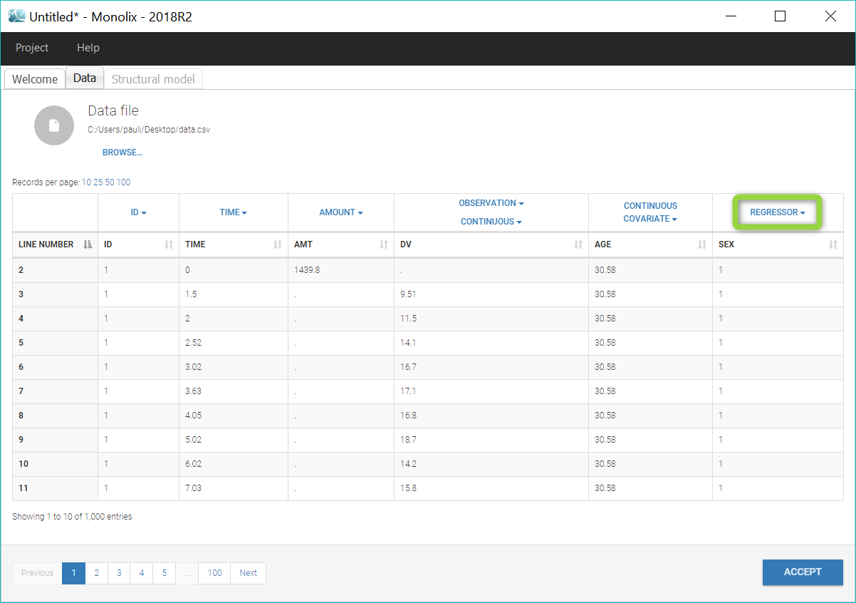
Step 2: In the model file shown below, the covariate SEX is passed as input argument and designated as being a regressor. Two parameters VM (for male) and VF (for female) are given as input, to be used as the volume V depending on the SEX. The use of VM or VF depending on the SEX value is defined in the EQUATION: block, before V is used (for instance in a simple (V,Cl) model):
[LONGITUDINAL]
input = {Cl, VM, VF, SEX}
SEX = {use=regressor}
EQUATION:
if SEX==0
V = VM
else
V = VF
end

Cc = pkmodel(Cl, V)

OUTPUT:
output = {Cc}
Step 3: The distribution of the parameters VM and VF is set as usual in the GUI. A different typical population value and a different standard deviation of the random effects will be estimated for males and females.
Note: As SEX has been tagged as a regressor, it is not available as a covariate in the GUI. If a covariate effect of SEX on another parameter is needed, the column SEX can be duplicated in the dataset so that the duplicate can be tagged as a covariate.
Covariate-dependent standard deviation
This video shows a variation of the previous solution, where only the standard deviation of the random effect of a parameter is covariate-dependent, while the fixed effect is not affected.
Transforming a continuous covariate into a categorical covariate
The Monolix GUI allows to discretize a continuous covariate in order to handle it as a categorical covariate in the model, using binary 0/1 values.
4.2.6.Inter occasion variability (IOV)
- Introduction
- Occasion definition in a data set
- Cross over study
- Occasions with washout
- Occasions without washout
- Multiple levels of occasions
Objectives: learn how to take into account inter occasion variability (IOV).
Projects: iov1_project, iov1_Evid_project, iov2_project, iov3_project, iov4_project
Introduction
A simple model consists of splitting the study into K time periods or occasions and assuming that individual parameters can vary from occasion to occasion but remain constant within occasions. Then, we can try to explain part of the intra-individual variability of the individual parameters by piecewise-constant covariates, i.e., occasion-dependent or occasion-varying (varying from occasion to occasion and constant within an occasion) ones. The remaining part must then be described by random effects. We will need some additional notation to describe this new statistical model. Let
- \(\psi_{ik}\) be the vector of individual parameters of individual i for occasion k, where \(1\leq i \leq N\) and \(1\leq k \leq K\).
- \({c}_{ik}\) be the vector of covariates of individual i for occasion k. Some of these covariates remain constant (gender, group treatment, ethnicity, etc.) and others can vary (weight, treatment, etc.).
Let \(\psi_i = (\psi_{i1}, \psi_{i2}, \ldots , \psi_{iK})\) be the sequence of K individual parameters for individual i. We also need to define:
- \(\eta_i^{(0)}\), the vector of random effects which describes the random inter-individual variability of the individual parameters,
- \(\eta_{ik}^{(1)}\), the vector of random effects which describes the random intra-individual variability of the individual parameters in occasion k, for each \(1\leq k \leq K\).
Here and in the following, the superscript (0) is used to represent inter-individual variability, i.e., variability at the individual level, while superscript (1) represents inter-occasion variability, i.e., variability at the occasion level for each individual. The model now combines these two sequences of random effects:
\(h(\psi_{ik}) = h(\psi_{\rm pop})+ \beta(c_{ik} – c_{\rm pop}) + \eta_i^{(0)} + \eta_{ik}^{(1)} \)
Remark: Individuals do not need to share the same sequence of occasions: the number of occasions and the times defining the occasions can differ from one individual to another.
Occasion definition in a data set
There are two ways to define occasions in a data set:
- Explicitly using an OCCASION column. It is possible to have, in a data set, one or several columns with the column-type OCCASION. It corresponds to the same subject (ID should remain the same) but under different circumstances, occasions. For example, if the same subject has two successive different treatments, it should be considered as the same subject with two occasions. The OCC columns can contain only integers.
- Implicitly using EVID column. If there is an EVID column with a value 4 then Monolix defines a washout and creates an occasion. Thus, if there are several times where EVID equals 4 for a subject, it will create the same number of occasions. Notice that if EVID equals 4 happens only once at the beginning, only one occasion will be defined and no inter occasion variability would be possible.
There are three kinds of occasions
- Cross over study: In that case, data is collected for each patient during two independent treatment periods of time, there is an overlap on the time definition of the periods. A column OCCASION can be used to identify the period. An alternative way is to define an EVID column starting for all occasions with EVID equals 4. Both types of definition will be presented in the iov1 example.
- Occasions with washout: In that case, data is collected for each patient during one period and there is no overlap between the periods. The time is increasing but the dynamical system (i.e. the compartments) is reset when the second period starts. In particular, EVID=4 indicates that the system is reset (washout) for example, when a new dose is administrated.
- Occasions without washout: In that case, data is collected for each patient during one period and there is no overlap between the periods. The time is increasing and we want to differentiate periods in terms of occasions without any reset of the dynamical system. Multiple doses are administrated to each patient. each period of time between successive doses is defined as a statistical occasion. A column OCCASION is therefore necessary in the data file to define it.
Cross over study
- iov1_project (data = ‘iov1_data.txt’, model = ‘lib:oral1_1cpt_kaVk.txt’)
In this example, PK data is collected for each patient during two independent treatment periods of time (each one starting at time 0). A column OCCASION is used to identify the study:
This column is defined using the reserved keyword OCCASION. Then, the model associated to the individual parameter is as presented below
 First, to define the variability of each parameter on each level, you just have to go on the good level, and you’ll see the associated random effects on each level. On the figure above, we see that all parameters have variability on the ID level, which means that all parameters have inter-individual variability. On the figure below, we see the OCC level. In the presented case, only the volume V has inter-study variability and thus inter occasion variability. Thus, this is the only one having variability on the occasion level.
In terms of covariates, we then see two parts as displayed below. We see the covariates
- associated to the level ID (in green). It corresponds to all the covariates that are constant for each subject.
- associated to the level OCC (in blue). It corresponds to all the covariates that are constant for each occasion but not on each subject.
In the presented case, the treatment TRT varies for each individual. It contains inter-occasion information and is thus displayed with the occasion level. On the other hand, the SEX is constant for each subject. It contains then inter-individual information but no inter-occasion information. It is then displayed with the ID level.
 What is the impact?
Covariates can be associated to the parameter if and only if their level of variability is coherent with the level of variability of the parameter. In the presented case,
- TRT has inter-occasion variability. It can only be used with the parameter V that has inter-occasion variability. The two other parameters have only inter-individual variability and can therefore not use this TRT information. The interface is greyed and the user can not add this covariate to the parameters ka and Cl.
- SEX has only inter-individual variability. It can therefore be associated to any parameter that has inter-individual variability.
The population parameters now include the standard deviations of the random effects for the 2 levels of variability (omega is used fo IIV and gamma for IOV):
Two important features are proposed in the plots. Firstly, in the individual fits, you can split or merge the occasions. When split is done, the name of the subject-occasion is the name of the subject, #, and the name of the occasion.
 |
 |
|---|
Secondly, you can use the occasion to split the plots
- iov1_Evid_project (data = ‘iov1_Evid_data.txt’, model = ‘lib:oral1_1cpt_kaVk.txt’)
Another way to describe this cross over study is to use EVID=4 as explained in the data set definition. In that example, the EVID creates a washout and another occasion.

Occasions with washout
- iov2_project (data = ‘iov2_data.txt’, model = ‘lib:oral1_1cpt_kaVk.txt’)
The time is increasing in this example, but the dynamical system (i.e. the compartments) is reset when the second period starts. Column EVID provides some information about events concerning dose administration. In particular, EVID=4 indicates that the system is reset (washout) when a new dose is administrated
Monolix automatically proposes to define the treatment periods (between successive resetting) as statistical occasions and introduce IOV, as we did in the previous example. We can display the individual fit by splitting each occasion for each individual
Or by merging the different occasions in a unique plot for each individual:
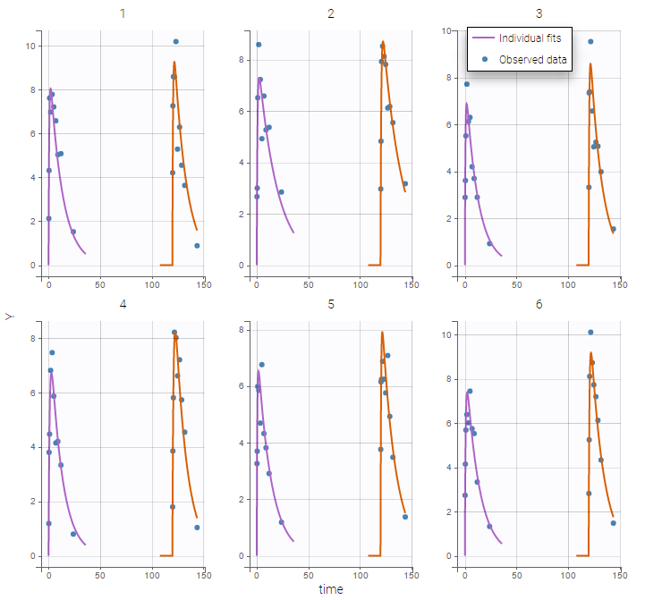 Remark: If you are modeling a PK as in this example, the washout implies that the occasions are independent. Thus, the cpu time is much faster as we do not have to compute predictions between occasions.
Occasions without washout
- iov3_project (data = ‘iov3_data.txt’, model = ‘lib:oral1_1cpt_kaVk.txt’)
Multiple doses are administrated to each patient. We consider each period of time between successive doses as a statistical occasion. A column OCCASION is therefore necessary in the data file.
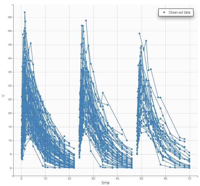 We can color the observed data by their occasion to have a better representation
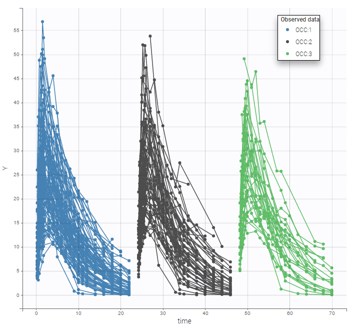
The model for IIV and IOV can then be defined as usual. The plot of individual fits allows us to check that the predicted concentration is now continuous over the different occasions for each individual:
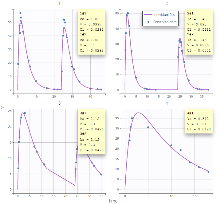
Multiple levels of occasions
- iov4_project (data = ‘iov4_data.txt’, model = ‘lib:oral1_1cpt_kaVk.txt’)
We can easily extend such an approach to multiple levels of variability. In this example, columns P1 and P2 define embedded occasions. They are both defined as occasions:

We then define a statistical model for each level of variability.

4.2.7.Inter-occasion variability and effect of guar gum on alcohol concentration in blood
This case study uses the MonolixSuite to analyze and model the absorption and elimination of alcohol with or without a dietary additive of guar gum. It focuses in particular on the modeling of inter-occasion variability.
Guar gum, also called guaran, is a polysaccharide extracted from guar beans. As a natural polymer, it has been used for many years as an emulsifier, thickener, and stabilizer in the food industry. In the pharmaceutical sector, guar gum and guar-gum based systems are frequently studied for the development of controlled-released formulations and colon targeted drug delivery systems, as guar gum can protect active molecules from the enzymes and pH in the stomach and small intestine and it can be degraded by intestinal bacteria in the colon. [Aminabhavi, T. M., Nadagouda, M. N., Joshi, S. D., & More, U. A. (2014). Guar gum as platform for the oral controlled release of therapeutics. Expert Opinion on Drug Delivery, 11(5), 753–766.]
Moreover, guar gum may affect the bioavailability of concomitantly administered substances due to its effect on the rate of gastrointestinal transit and gastric emptying.
The goal of this case study is then to assess the effect of guar gum on the absorption and bioavailability of alcohol.
Outline:
Data set
The data has been published in:
Practical Longitudinal Data Analysis, David J. Hand, Martin J. Crowder, Chapman and Hall/CRC, Published March 1, 1996
It is composed of measurements of blood alcohol concentrations in 7 healthy individuals. All subjects took alcohol at time 0 and gave a blood sample at 14 times over a period of 5 hours. The whole procedure was repeated at a later date but with a dietary additive of guar gum. The two different periods of time are encoded in the data with overlapping times, both starting at time 0.
Although the precise amount of ingested alcohol is unknown, for this case study we assume each amount to be 10g (standard drink).
Data exploration in Datxplore
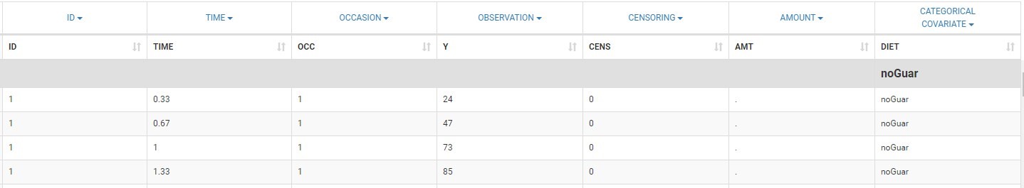
The data is loaded in Datxplore to explore it graphically. It appears in the Data tab as above. The time is in hours, the alcohol concentration in the column Y is in mg/L, and the amount in AMT is in mg. Censored observations are indicated with the column CENS tagged as CENSORING.
The two periods of measurements, during which the subjects have received or not guar gum in addition to alcohol are distinguished with the column OCC, which is automatically recognized as OCCASION. In addition, I use the column DIET that I tag as CATCOV to indicate which occasion corresponds to the addition of guargum. This column contains 2 strings: noGuar for occasion 1 and withGuar for occasion 2.
In the Plots tab, the plot of alcohol concentration vs time in log-scale seen below suggests to use a one-compartment model with a first-order absorption. A non-linear elimination appears for some individuals, but the data might not be sufficient to capture it. Thus a linear elimination should be tried as a first model.
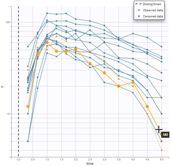
The different occasions can be visualized in several ways. First, hovering on a curve highlights the curve in solid yellow and the curve corresponding to the other occasion from the same subject in dashed yellow, as on the figure above.
Second, OCC is available for stratification along with the covariate DIET in the “Stratify” panel , and can thus be used for splitting, coloring or filterting. Below are for example the subplots of the data split by OCC and colored by ID. Each subject-occasion is assigned a color, with matched color shades for subject-occasions corresponding to the same subject. This is convenient to compare at a glance the two occasions for all subjects. The inter-individual variability seems mostly reproduced from one occasion to the other, and concentration levels seem slightly higher for OCC=2.
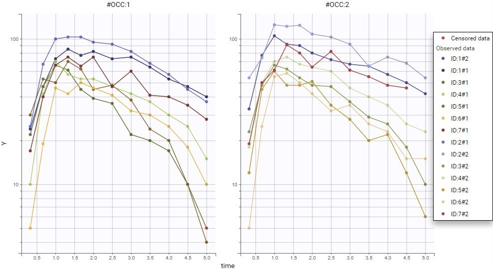
This global trend can be confirmed in linear scale below. Here the plot is colored by DIET, whose categories are matched with OCC: DIET=noGuar corresponds to OCC=1 and DIET=withGear to OCC=2. Thus, the main inter-occasion variability seen in the data seems to be explained by the covariate DIET.
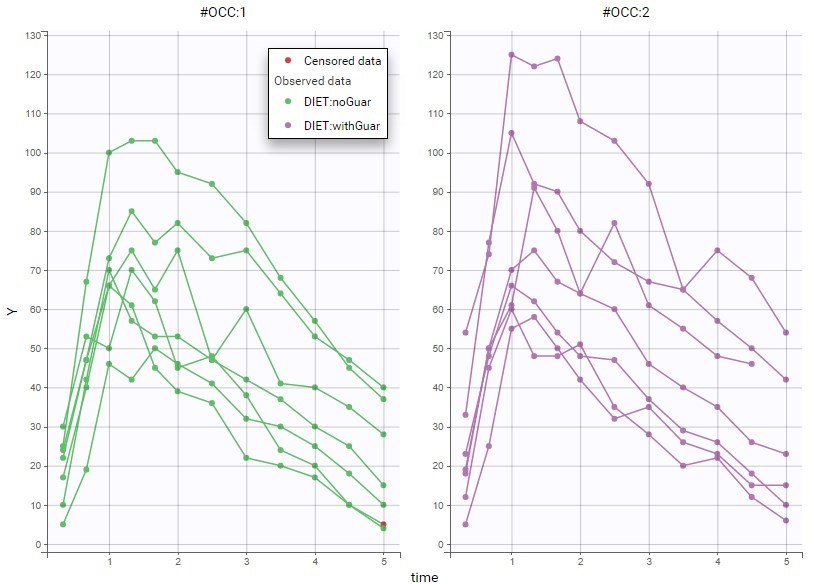
First analysis in PKanalix
Non-compartmental analysis
As a first analysis, we can check the difference in PK parameters for the two occasions with non-compartmental analysis (NCA) in PKanalix. After loading the previously saved Datxplore project in PKanalix, the following settings are chosen:
- extravascular administration,
- “linear up log down” integral method,
- “missing” for blq after Tmax (censored observations after Tmax are not used in the analysis).
The “Check lambda_z” panel, seen below, allows to check the regressions estimating the elimination slope. The default “adjusted R2” rule selects for each individual the optimal number of points used in the regression to get the best regression. While the plots allow to adjust the selection of points for some individuals, it is not necessary here. The plots already show some variability between individuals in the estimated lambza_z.
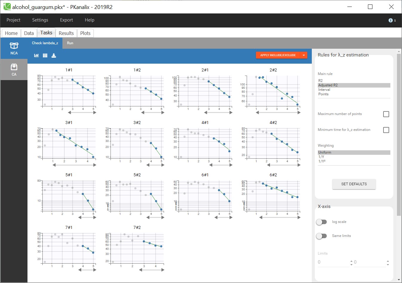
Running the NCA gives the lambda_z and other PK parameters for each individual. In the “Plot” tab, the plot of individual parameters vs. covariates is convenient to visualize the variability in the parameters and compare the distributions without and with guar gum. Here the following parameters have been selected: AUCINF_pred, Cl_F_pred, Cmax, HL_Lambda_z, Tmax:
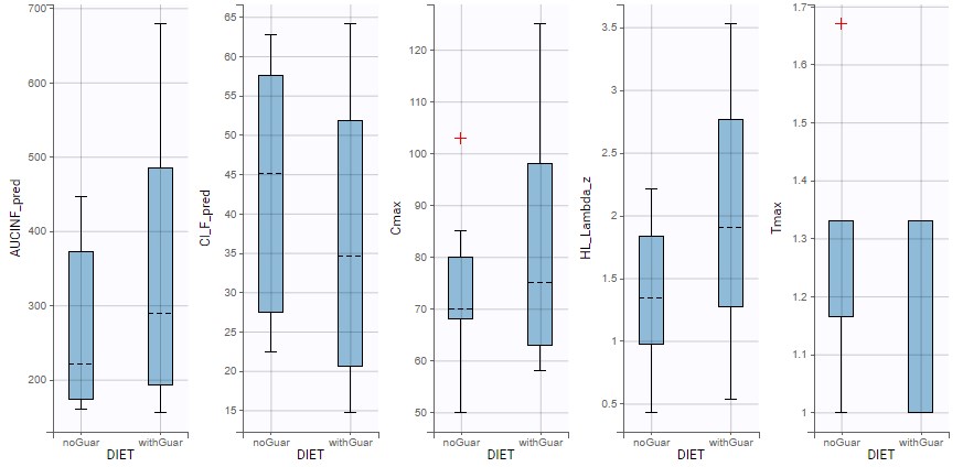
Some difference can be seen between the two conditions for the half-life, the apparent clearance and Cmax, however the parameters also show large variability within each dietary condition.
Compartmental analysis in PKanalix
Next, a compartmental analysis (CA) can be run to estimate a compartmental model and compare the estimated parameters between the two conditions. PKanalix considers that the subject-occasions are independent, thus the parameters are optimized independently on each individual and on each occasion. This allows to check easily if different values are estimated for the two occasions.
Choosing a one-compartment model with a first-order absorption and a linear elimination gives the following individual fits (after choosing initial values with the “aut-init” button):
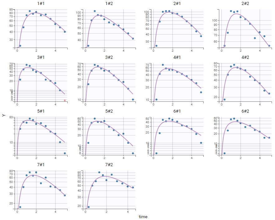
The absorption phase is not really well captured. Zooming on this phase can help confirm that the absorption should be delayed. Choosing the same model as before but with a lag time before the absorption now gives good individual fits:
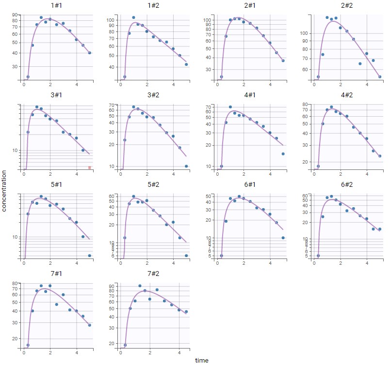 In the plot Individual parameters vs. covariates, the estimated individual parameters show different distributions across the two conditions of DIET, in particular for ka, V and k:
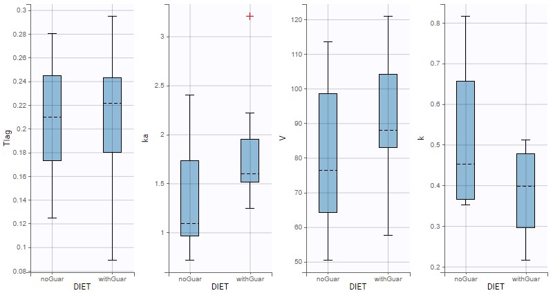
Since the data size is small, it is not clear whether these differences are significant. The effect of DIET on the alcohol kinetics can be assessed more precisely with a detailed population analysis in Monolix.
Moreover, the bioavailability is not explicitly taken into account by this model, because it is not identifiable with only extravascular administrations, so it is included in the apparent volume V. In Monolix, it is possible to use more complex models than the simple PK models from the library, and in particular to add the bioavailability explicitly, allowing to assess in a more meaningful way whether guar gum could have an effect on the relative bioavailability depending on the value of DIET.
Therefore, we export the compartmental model from PKanalix to Monolix.
Population modelling in Monolix
This opens a Monolix project in which the data and the structural model are set up like in PKanalix.
In “Statistical model & Tasks”, the “Individual model” part is now split in two. The part on the left at the ID level describes the inter-individual variability (IIV), and includes by default a random effect for each parameter. The part on the right (highlighted in the figure below) is dedicated to the OCC variability-level, where it is possible to add random effects at the inter-occasion level: this would create inter-occasion variability (IOV). Since DIET varies from one occasion to another, it appears in this panel to explain part of the inter-occasion variability with a covariate effect. The boxes for adding covariate effects are greyed out, because at this step there is no inter-occasion variability. It is only possible to add covariate effects at the occasion level on parameters that either have inter-occasion variability with random effects at the occasion level, or parameters that have no random effects at the id and occasion levels.
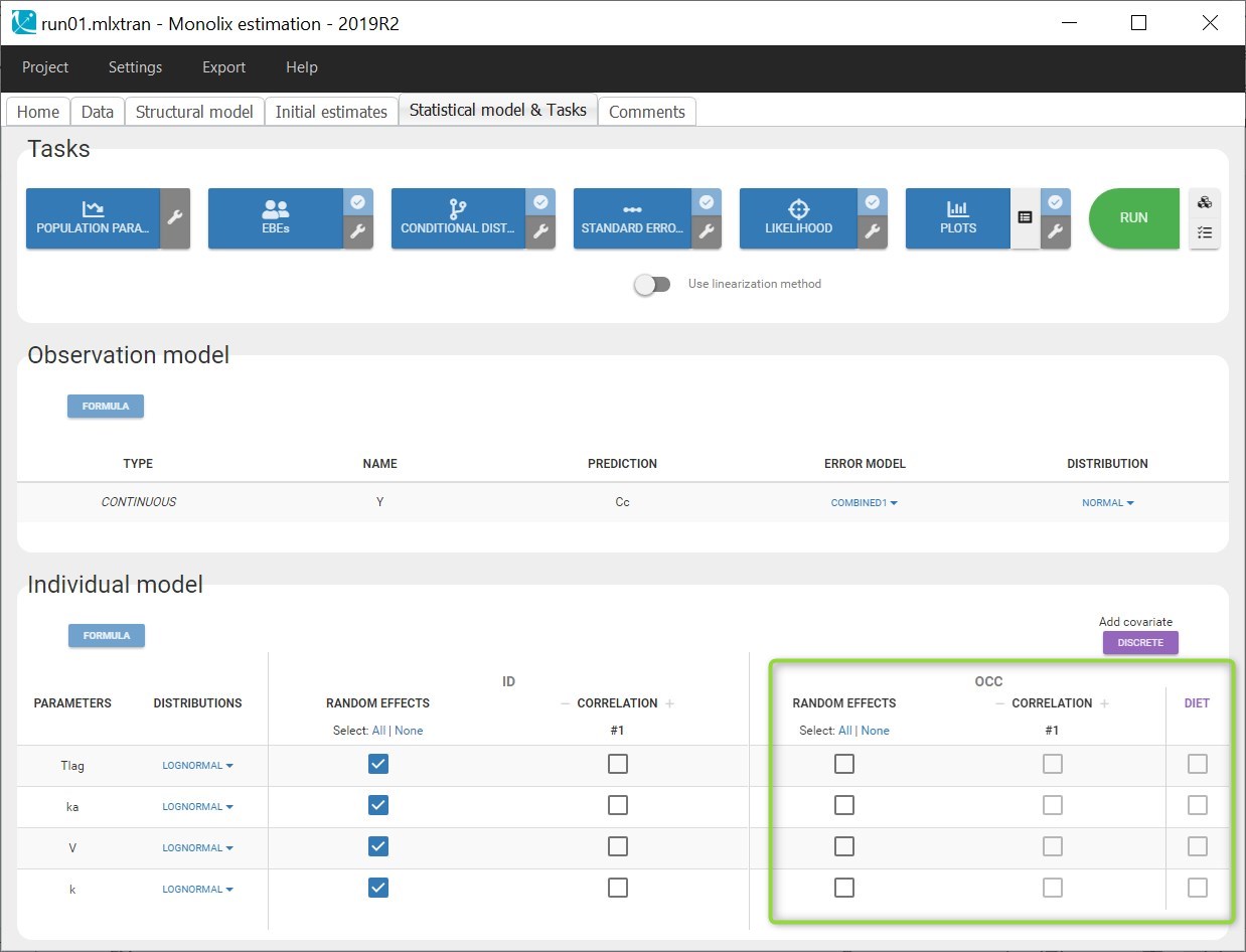
Model without inter-occasion variability
The first step in this worklow aims at validating the structural model without taking into account differences between the occasions. Thus we keep the statistical model to default, select all tasks in the scenario and save the project as run01.mlxtran.
Estimating this model does not show misspecifications on the plot of Observations vs Predictions in log-log scale:
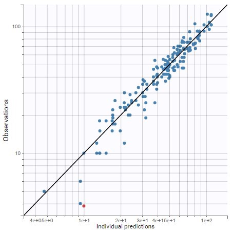
All parameters are estimated with a good confidence, except omega_ka which is small and with a high rse:
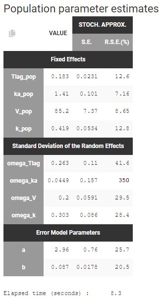
On the individual fits seen below, disabling the option “Split occasions” in “Display” allows to visualize the two occasions on the same plot for each individual. The observed data can be colored by occasion or equivalently by DIET in Stratify.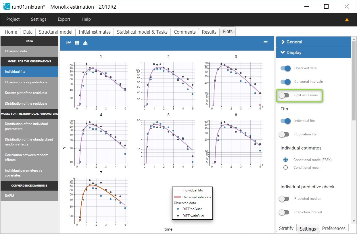
In this case, the predictions are identical for both occasions and overlap, since no inter-occasion variability is taken into account in the model. The prediction curves are displayed in purple for the first occasion and orange for the second, by default the curve for the first occasion on top, except for the last individual for which the second occasion is on top because it corresponds to a smaller observation period.
The individual fits shows that capturing both occasions with the same prediction is not possible, because there are small non-random variations from one occasion to another, as seen during the data exploration. This could corresponds to variability in the parameters between the occasions, that can be taken into account in the “Statistical model & Tasks” tab, by adding some random effects at the inter-occasion level or defining a covariate effect of DIET. We will first focus on the random effects.
Model with relative bioavailability and unexplained inter-occasion variability
Each parameter can be modelled with IIV, IOV or both. Physiological considerations can help deciding if a parameter should have variability at each level or not. But in the absence of clear physiological knowledge, a possible approach is also to add a random effect at the occasion level on each parameter for which variability may be relevant, and check if the estimated standard deviation of the random effect is small.
In this case, all parameters may show some inter-occasion variability. Indeed, the elimination can easily show some variations between different periods, and the dietary additive of guar gum might change the values of the parameters Tlag and ka characterizing the absorption. The volume V is unlikely to vary much for one occasion to another, however in this case V corresponds to the apparent volume, that includes the bioavailability of alcohol, which may vary with guar gum. Thus, it would be possible to set a random effect for IOV on V, or alternatively to modify the structural model to include explicitly the bioavailability, and add the random effect at the occasion level on the bioavailability instead of the volume. This is what we are going to do.
Before modifying the structural model, we use the last estimates as new initial values to facilitate the estimation for the next run.
Then, we open the structural model in the editor, and add an argument p=F in the pkmodel macro. This means that the proportion of absorbed drug will be defined by the parameter F, that should also be added in the input list:
[LONGITUDINAL]
input = {Tlag, ka, V, k, F}

EQUATION:
; PK model definition
Cc = pkmodel(Tlag, ka, V, k, p=F)

OUTPUT:
output = Cc
This modified model is then saved under a new name. The compile button is convenient to check that there is no syntax error. The new model can then be loaded in Monolix instead of the previous one.
After loading the model, Monolix brings us to the “Check initial estimates” tab to choose a good initial value for F_pop. Here F is not the absolute bioavailability, but it corresponds to a relative bioavailability between the individuals. Thus F_pop is the reference value for the bioavailability, and it should be fixed to 1. This can be done in the list of the initial estimates, by changing the estimation method for F_pop to “Fixed”:
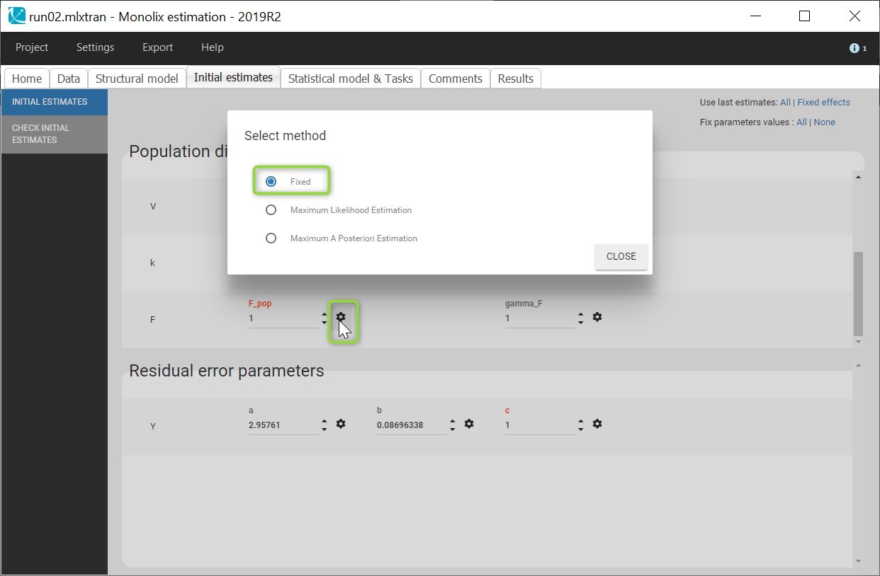
Now that the model includes the relative bioavailability explicitly, we can consider IOV for F instead of for V. Since V and F are not identifiable together, we should not include IIV for F while there is already IIV for V.
Clicking on Formula displays the model for the individual parameters. For instance, the model for Tlag now includes a random effect eta_OCC_Tlag in addition to the random effect eta_ID_Tlag:
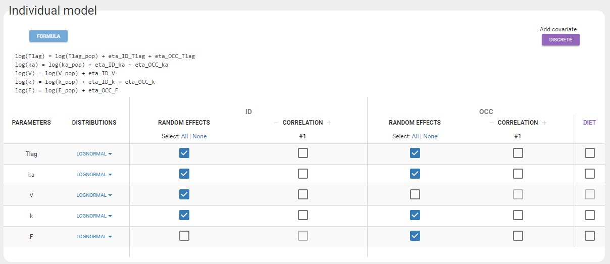
This project is saved as run02.mlxtran and all tasks are run.
The table of population parameters now include the standard deviations of the new random effects at the OCC level, which are called gamma:
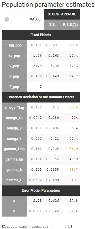
There a few high rses for the standard deviations of the random effects, because it is not possible to identify well all the random effects with such a small dataset. The random effects with the smallest standard deviations could probably be removed, such as omega_ka or gamma_F. In a later step, we will check more precisely which random effects should be removed. For now, we will first check the relationships between the random effects and the covariate DIET.
On the individual fits, there are now different individual predictions for each occasion. The colors associated to each value of DIET for the observations can be changed in “Stratify” to match the colors of the predictions. The predictions from occasion 1 are in purple, they correspond to the first category noGuar. The second category withGuar corresponds to the second occasion with orange predictions.
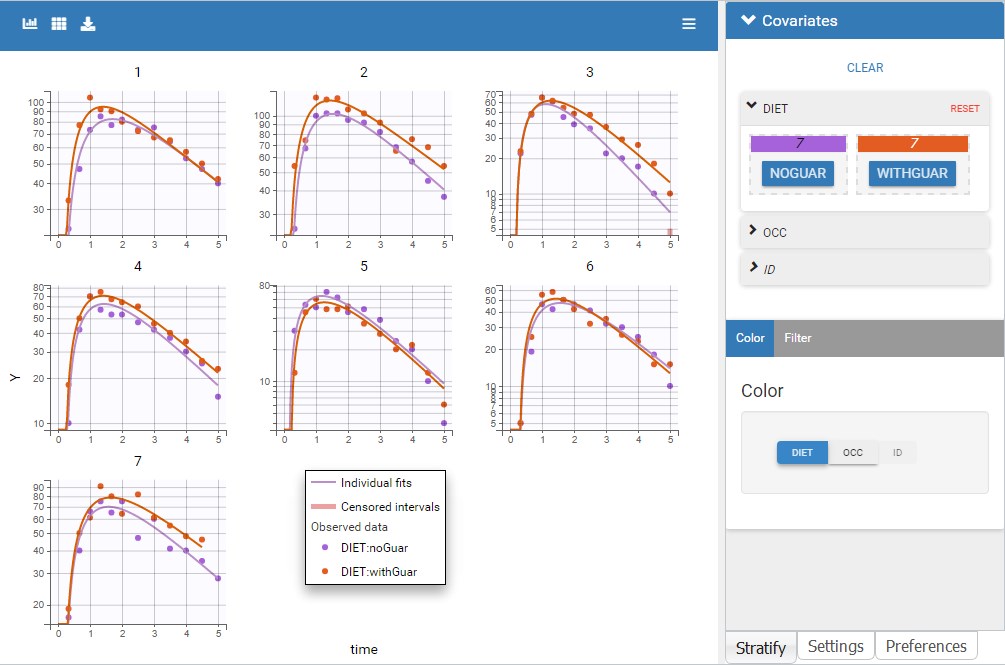
After clicking on Information, the individual parameter values appear on the plots for each occasion (for example here for the two first individuals):
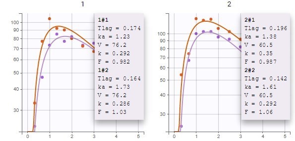
For V, which has only IIV, a single value is estimated for each individual across both occasions. For F, which has only IOV, it is important to note that estimated individual random effects from the distribution defined by gamma_F are independent across ids and occasions, and take into account the fact that F is slightly different for all subject-occasions. So a different value is estimated for each subject-occasion. Thus, the inter-occasion variability represents also an inter-individual variability. For parameters that have both IIV and IOV (Tlag, ka and k), the variability at the id level represents the additional variability between individuals that is common across both occasions.
The individual fits show that the IOV allows to properly capture the observations for each subject-occasion, and the predicted alcohol concentration seems usually higher when individuals have taken guar gum, except for ids 5 and 6. Let’s check this with the other diagnostic plots.
Assessing the effect of guar gum on alcohol’s PK
First, the plot of individual parameters vs covariates can be used to compare the distributions of each parameters across the two occasions.
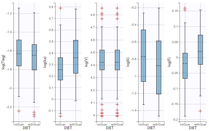
Notable differences appear for ka, k and F. The kinetics with guar gum exhibit higher absorption rates and bioavailability, and smaller elimination rates. We can try to implement one or several of these differences in the model with a covariate effect, starting with the hypothesis that guar gum could affect the bioavailability of alcohol.
The statistical tests in Results show that these differences do not correspond to a significant correlation between eta_ka and DIET, but there is a significant correlation with eta_k, and a slightly significant correlation with eta_F. The lack of significance for ka and F is explained by the small size of the data which affects the p-values.
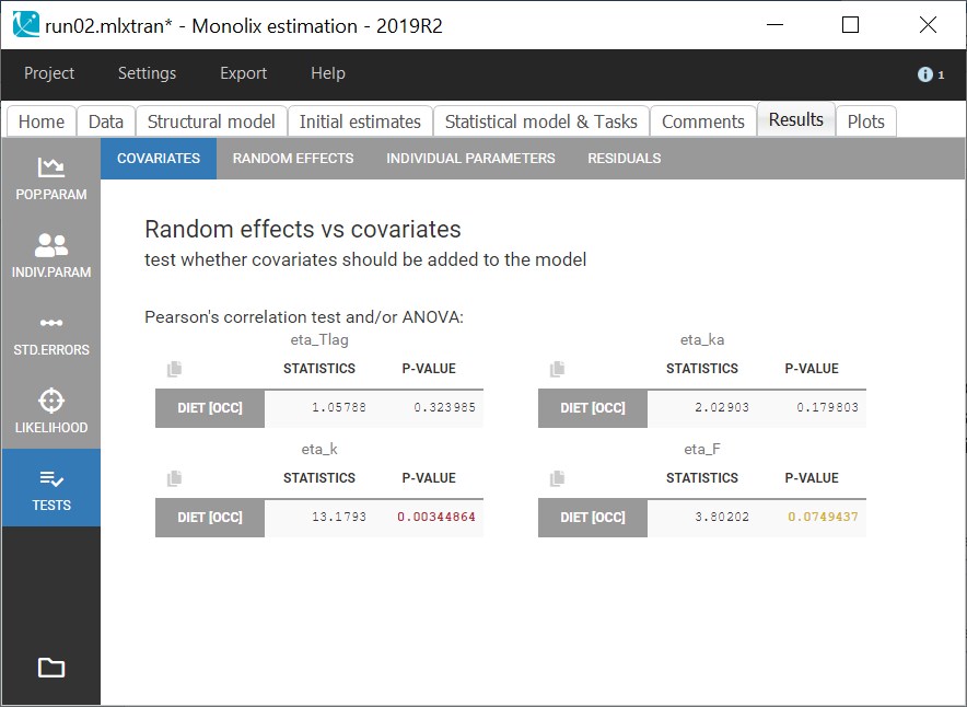
Second, we can have a look at the VPC split by DIET. Here, the prediction intervals are based on simulations that use the IOV included in the model, which is independent from DIET. Thus the prediction intervals are almost identical on each plot, while the empirical curves differ with DIET.
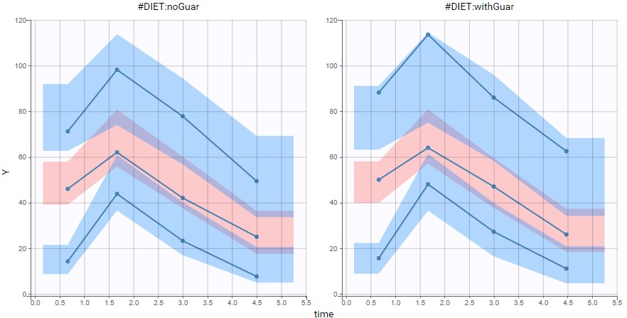
With the 4 bins computed by default, empirical curves are well captured by the prediction intervals, so with this size of data, the small differences caused by guar gum do not cause a visible discrepancy of the model, but when setting the number of bins to 6 (see below), a small discrepancy appears in the absorption phase. Although we should keep in mind that the empirical percentiles represent only a small number of individuals, this is a hint that it could be relevant to take into account an effect of guar gum on the absorption or the bioavailability.
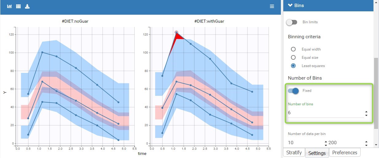
Model with inter-occasion variability and occasion-varying covariate effect
As a result of this diagnosis, we can now adjust the model, after using the last estimates as new initial values. Based on the diagnostic plots and the biological knowledge on possible mechanisms for the effect of guar gum, we will try to explain part of the IOV by adding a covariate effect of DIET on F. We save this modified project as run03.mlxtran and run all tasks.
The new parameter beta_F_DIET_withGuar is estimated to a small value (0.08) but with a good standard error, and it results in a small decrease of gamma_F (from 0.07 to 0.034):
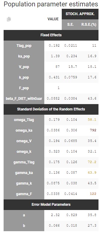
In the statistical tests, the p-value for the Wald test, which checks whether the parameter is close to 0, is small but the test is not quite significant. In addition, the correlation between F and DIET is significant:
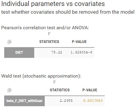
The diagnostic plot also show that this correlation is strong:
Therefore the covariate effect is relevant and should not be removed from the model.
Moreover, the -2*LL and BICc for run03.mlxtran are slightly smaller than run02.mlxtran (2 points of difference), showing that the modified model still captures the data as well as the previous run. This can be seen easily by comparing the runs in Sycomore:
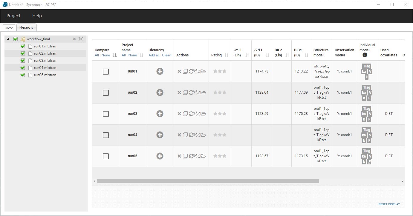
Estimation without simulated annealing
Finally, in the next step we are going to check more precisely whether some random effects are not well estimated and should be removed.
For the next run, we are going to modify the settings of SAEM to disable the simulated annealing:
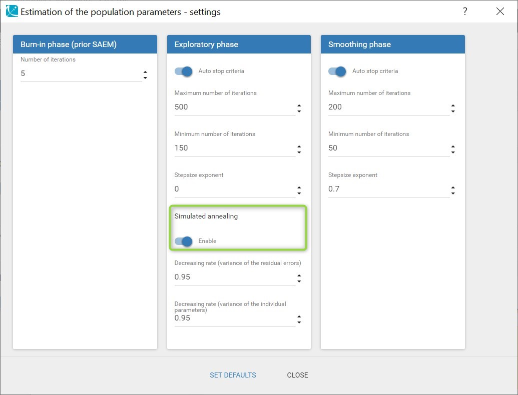
This option is explained in details in this video. Briefly, it constrains the variance of the random effects to decrease slowly during the estimation, in order to explore a large parameter space to avoid getting stuck in a local maximum. A side-effect of the simulated annealing is that it may keep the omega values artificially high, and prevent the identification of parameters for which the variability is in fact zero. This leads to large values in the standard errors. So when large standard errors are estimated for random effects, like it is the case here for omega_ka and gamma_F, it is recommended to disable the simulated annealing once the estimated parameters are close to the solution.
Before changing the settings, the last estimates should be used as new initial values to start really close to the solution. The modified project is saved as run04.mlxtran and SAEM is run. In the graphical report, omega_ka and gamma_F now decrease to a very small value:
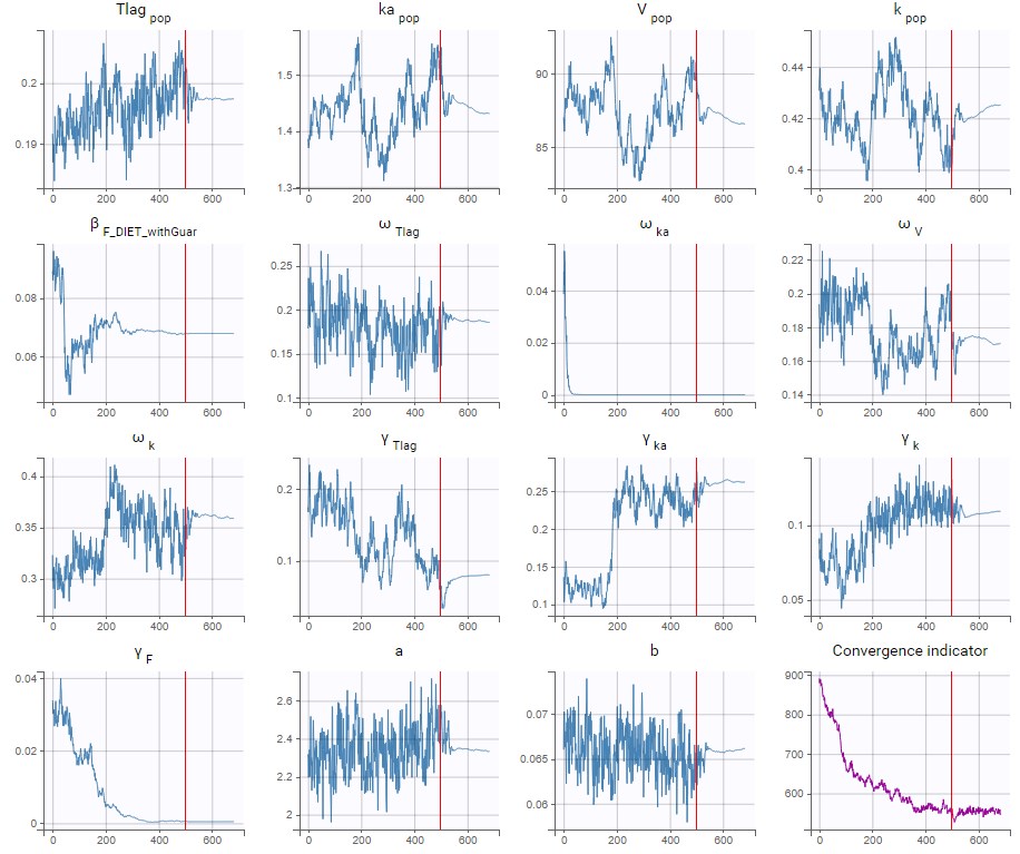
This confirms that there is not enough information in the data to identify the distributions for ka and F. Therefore, we can use the last estimates and then remove the IIV on ka and the IOV on F. The IOV on F can be removed while keeping the covariate effect of DIET, because F has also no IIV.
After doing this, we run the whole scenario again for the new project run05.mlxtran. All the parameters are now estimated with quite good standard errors, considering the small size of the data:
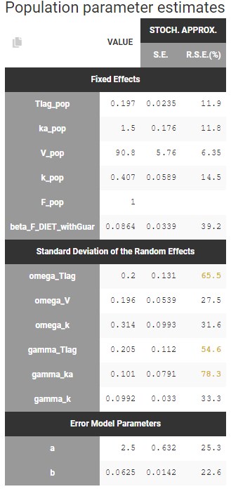
With the covariate effect on DIET on F, the discrepancy in the VPC for the occasions with guar gum is slightly smaller but still present, and is likely due to the variability in the data:
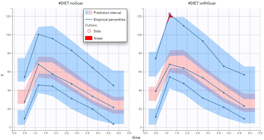
This run is the final model. Despite the small size of the data, it is able to take into account IIV and IOV, and to explain a modest part of the inter-occasion variability in bioavailability of alcohol by the effect of guar gum.
4.2.8.Mixture of distributions
- Introduction
- Mixture of distributions based on a categorical covariate
- Mixture of distributions based on unsupervised classification with a latent covariate
Objectives: learn how to implement a mixture of distributions for the individual parameters.
Projects: PKgroup_project, PKmixt_project
Introduction
Mixed effects models allow us to take into account between-subject variability.
One complicating factor arises when data is obtained from a population with some underlying heterogeneity. If we assume that the population consists of several homogeneous subpopulations, a straightforward extension of mixed effects models is a finite mixture of mixed effects models.
There are two approaches to define a mixture of models:
- defining a mixture of structural models (via a regressor or via the bsmm function) –> click here to go to the page dedicated to this approach,
- introducing a categorical covariate (known or latent). This approach is detailed here.
The second approach assumes that the probability distribution of some individual parameters vary from one subpopulation to another one. The introduction of a categorical covariate (e.g., sex, phenotype, treatment, status, etc.) into such a model already supposes that the whole population can be decomposed into subpopulations. The covariate then serves as a label for assigning each individual to a subpopulation.
In practice, the covariate can either be known or not. If it is unknown, the covariate is called a latent covariate and is defined as a random variable with a user-defined number of modalities in the statistical model. Differences in estimation and diagnosis methods appear to deal with this additional random variable: this difference represents a task of unsupervised classification.
Mixture models usually refer to models for which the categorical covariate is unknown and unsupervised classification is needed.
For the sake of simplicity, we will consider a basic model that involves individual parameters \((\psi_i,1\leq i \leq N)\) and observations \((y_{ij}, i \leq N, 1\leq j \leq n_i)\). Then, the easiest way to model a finite mixture model is to introduce a label sequence \((z_i , 1\leq i \leq N)\) that takes its values in \(\{1,2,\ldots,M\}\) such that \(z_i=m\) if subject i belongs to subpopulation m.
In some situations, the label sequence \((z_i , 1\leq i \leq N)\) is known and can be used as a categorical covariate in the model. If \((z_i)\) is unknown, it can be modeled as a set of independent random variables taking their values in \(\{1,2,\ldots,M\}\) where for \(i=1,2,\ldots, N\), \(P(z_i = m)\) is the probability that individual i belongs to group m. We will assume furthermore that the \((z_i)\) are identically distributed, i.e., \(P(z_i = m)\) does not depend on i for \(m=1, \ldots, M\).
Mixture of distributions based on a categorical covariate
- PKgroup_project (data = ‘PKmixt_data.txt’, model = ‘lib:oral1_1cpt_kaVCl.txt’)
The sequence of labels is known as GROUP in this project and comes from the dataset. It is therefore defined as a categorical covariate that classifies We can then assume, for instance different population values for the volume in the two groups and estimate the population parameters using this covariate model.
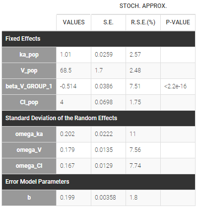
Then, this covariate GROUP can be used as a stratification variable and is very important in the modeling.
Mixture of distributions based on unsupervised classification with a latent covariate
A latent covariate is defined as a random variable, and the probability of each modality is part of the statistical model and is estimated as well. Methods for estimation and diagnosis are different. After the estimation, for each individual the categorical covariate is not perfectly known, only the probabilities of each modality are estimated.
Note also that latent covariates can be useful to model statistical mixtures of populations, but they provide no biological interpretation for the cause of the heterogeneity in the population since they do not come from the dataset.
Latent covariates can not be handled with IOV.
- PKmixt_project (data = ‘PKmixt_data.txt’, model = ‘lib:oral1_1cpt_kaVCl.txt’)
We will use the same data with this project but ignoring the column GROUP (which is equivalent to assuming that the label is unknown). If we suspect some heterogeneity in the population, we can introduce a “latent covariate” by clicking on the grey button MIXTURE.
 It is possible to change the name and the number of modalities of this latent covariate.
Remark: several latent covariates can be introduced in the model, with different number of categories.
We can then use this latent covariate lcat as any observed categorical covariate. Again, we can assume again different population values for the volume in the two groups by applying it on the volume random effect and estimating the population parameters using this covariate model. Proportions of each group are also estimated, plcat_1 which is the probability to have modality 1:
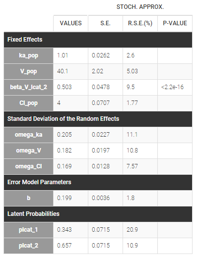
Once the population parameters are estimated, the sequence of latent covariates, i.e. the group to which belongs each subject, can be estimated together with the individual parameters, as the modes of the conditional distributions.
The sequence of estimated latent covariates lcat can be used as a stratification variable. We can for example display the VPC in the 2 groups:
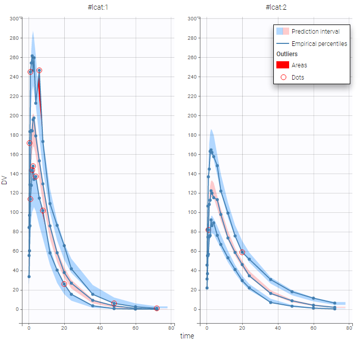
By plotting the distribution of the individual parameters, we see that V has a bimodal distribution
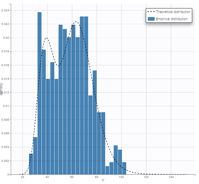
5.Tasks and results
Monolix tasks
Monolix allows a workflow with several tasks.
On the interface, one can see six different tasks
- POP. PARAM.: it corresponds to the estimation of the population parameters,
- EBEs: it corresponds to the estimation of the individual parameters using the conditional mode, i.e. the most probable individual parameters.
- CONDITIONAL DISTRIBUTION: It corresponds to the draws individual parameters based on the conditional distribution. It allows to compute the mean value of the conditional distribution.
- STD. ERRORS.: it corresponds to the calculation of the Fisher information matrix and standard errors. Two methods are proposed for it. Either using the linearization method or using the stochastic approximation. The choice between those methods is done with the “Use linearization method” toggle under the tasks.
- LIKELIHOOD: it corresponds to the explicit calculation of the log-likelihood. A specificity of the SAEM algorithm is that it does not explicitly compute the objective function. Thus, a dedicated task is proposed. Two methods are proposed for it. Either using the linearization method or using the importance sampling. The choice between those methods is done with the “Use linearization method” toggle under the tasks. This toogle is for both STD ERRORS and LIKELIHOOD tasks to be more relevant.
- PLOTS: it corresponds to the generation of the plots.
Also, different types of results are available in the form of plots and tables. The tasks can be run individually by clicking on the associated button, or you can define a workflow by clicking on the tasks to run (on the small light blue checks) and click on the play button (in green) as proposed on the figure below.
Notice that you can initialize all the parameters and the associated methods in the “Initial Estimates” frame as described here.
Moreover, Monolix includes a convergence assessment tool. It is possible to execute a workflow as defined above but for different, randomly generated, initial values of fixed effects.
Monolix results
All the output files are detailed here.
Monolix-R functions
Monolix is now proposed with an API leading to the possibility to have access to the project exactly by the same way as you would do with the interface. All the functions are described here.
5.1.Estimation tasks
5.1.1.Initialization
Parameter initial estimates and associated methods
- Initialization of the estimates
- What method can I use for the parameters estimations?
- How to initialize your parameters?
Initial values are specified for the fixed effects, for the standard deviations of the random effects and for the residual error parameters. These initial values are available through the frame “Initial estimates” of the interface as can be seen on the following figure. It is recommended to initialize the estimation to have faster convergence.

Initialization of the estimates
Initialization of the “Fixed effects”
The user can modify all the initial values of the fixed effects. When initializing the project, the values are set by default to 1. To change it, the user can click on the parameter and change the value

Notice that when you click on the parameter, an information is provided to tell what value is possible. The constraint depends on the distribution chosen for the parameter. For exemple, if the volume parameter V is defined as lognormal, its initial value should be strictly greater than 0. In that case, if you set a negative value, an error will be thrown and the previous parameter will be displayed.
When a parameter depends on a covariate, initial values for the dependency (named with \(\beta\) prefix, for instance beta_V_SEX_M to add the dependency of SEX, on parameter V) are displayed. The default initial value is 0. In case of a continuous covariate, the covariate is added linearly to the transformed parameter, with a coefficient \(\beta\). For categorical covariates, the initial value for the reference category will be the one of the fixed effect, while for all other categories it will be the initial value for the fixed effect plus the initial value of the \(\beta\), in the transformed parameter space. It is possible to define different initial values for the non-reference categories. The equations for the parameters can be visualized by clicking on button formula in the “Statistical model & Tasks” frame
Initialization of the “Standard deviation of the random effects”
The user can modify all the initial values of the standard deviations of the random effects. The default value is set to 1. We recommend to keep these values high in order for SAEM to have the possibility to explore the domain.
Initialization of the “Residual error parameters”
The user can modify all the initial values of the residual error parameters. There are as many lines as continuous outputs of the model. The default value depends on the parameter (1 for “a”, 0.3 for “b” and 1 for “c”).
What method can I use for the parameters estimations?
For all the parameters, there are several methods for the estimation
- “Fixed”: the parameter is kept to its initial value and so, it will not be estimated. In that case, the parameter name is set to orange.
- “Maximum Likelihood Estimation”: The parameter is estimated using maximum likelihood. In that case, the parameter name remains grey. This is the default option
- “Maximum A Posteriori Estimation”: The parameter is estimated using maximum a posteriori estimation. In that case, the user has to define both a typical value and a standard deviation. For more about this, see here. In that case, the parameter name is colored in purple.
To change the method, click on the right of the parameter as on the following.

A window pops up to choose the method as on the following figure

Notice that you have buttons to fix all the parameters or estimate all on the top right of the window as can be seen on the following figure
How to initialize your parameters?
On the use of last estimates
If you have already estimated the population parameters for this project, then you can use the “Use the last estimates” buttons to use the previous estimates as initial values. The user has the possibility to use all the last estimates or only the fixed effects. The interest of using only the fixed effects is not to have too low initial standard effects and thus let SAEM explore a larger domain for the next run.

Check initial fixed effects
When clicking on the “Check the initial fixed effects”, the simulations obtained with the initial population fixed effects values are displayed for each individual together with the data points, in case of continuous observations. It allows also an automatic initialization in case of a model of the PK library as described here.
5.1.1.1.Check initial estimates and auto init
Check initial fixed effects
The subtab “Check initial estimates” is part of the tab “Initial estimates“.
When clicking on the “Check the initial estimates”, the simulations obtained with the initial population fixed effects values and the individual designs (doses and regressors) are displayed for each individual together with the data points, in case of continuous observations. This feature is very useful to find some “good” initial values. Although Monolix is quite robust with respect to initial parameter values, good initial estimates speed up the estimation. You can change the values of the parameters on the bottom of the screen and see how the agreement with the data change. In addition, you can change the axis to log-scale and choose the same limit on all axes to have a better comparison of the individuals. When you are confident with the initial values, you should click on the “SET AS INITIAL VALUES” button on the top of the frame to validate the selection.
In addition, if you think that there are not enough points for the prediction (if there are a lot of doses for example), you can change the discretization and increase the number of points as displayed in the blue box of the figure.
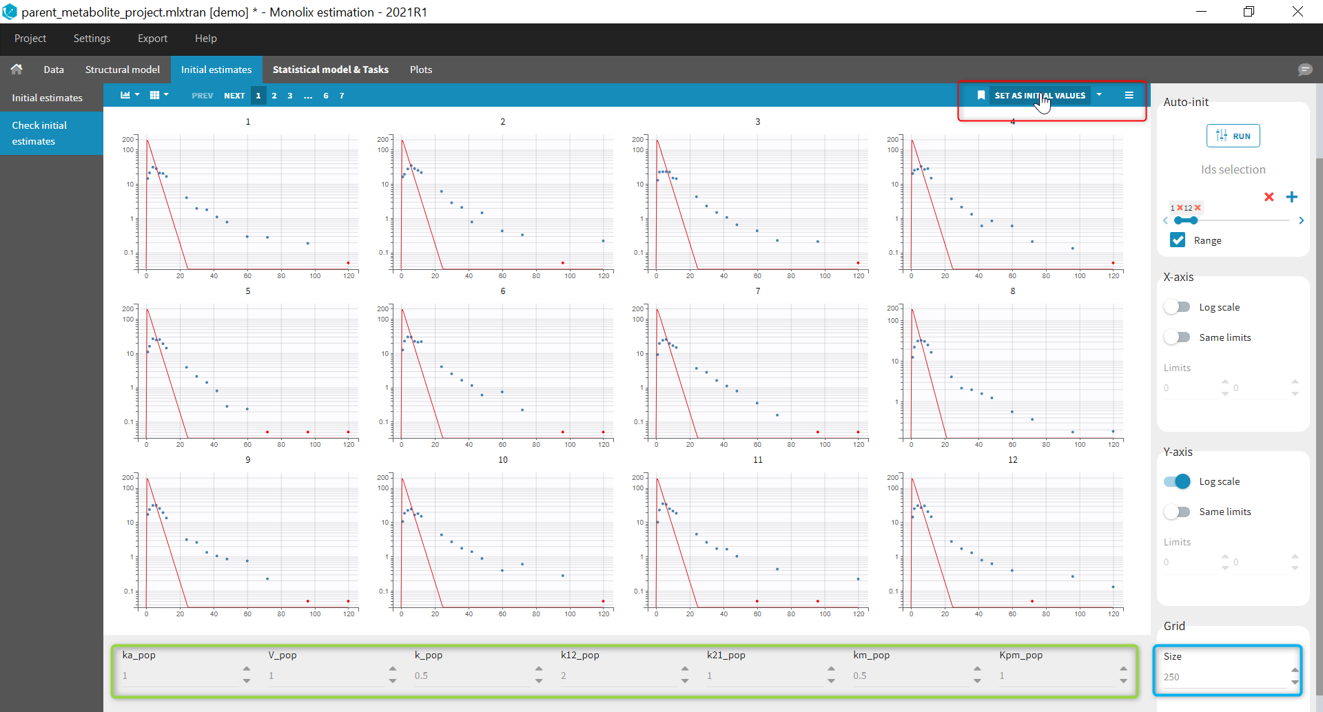
If several observation ids have been mapped to model outputs (for example a parent and a metabolite, or a PK and a PD observation), you can select which output to look at under the output section on the right:
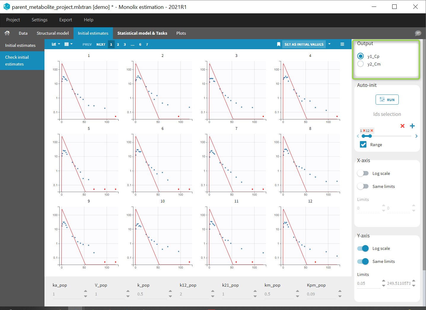
Using the reference in the “check initial estimates”
Starting from the 2019 version, it is possible to add a reference and thus change a parameter to see the impact of the variation of this parameter. In this example, we click on reference to use the current fit as reference and change k12 from 1 to 2 as can be seen on the following figure.
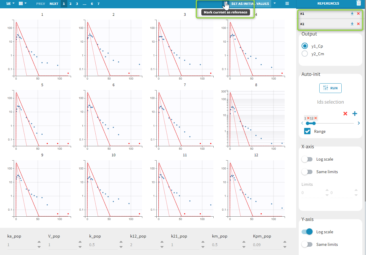
The solid red curve corresponds to the current curve and the dashed one corresponds to the reference. At any time, you can change the reference to use the current fit, and restore and delete the reference or delete all references by clicking on the icons at the top right of the frame.
Automatic initialization of the parameters
Starting from the 2021 version, an auto-init section appears on the right side of the frame:
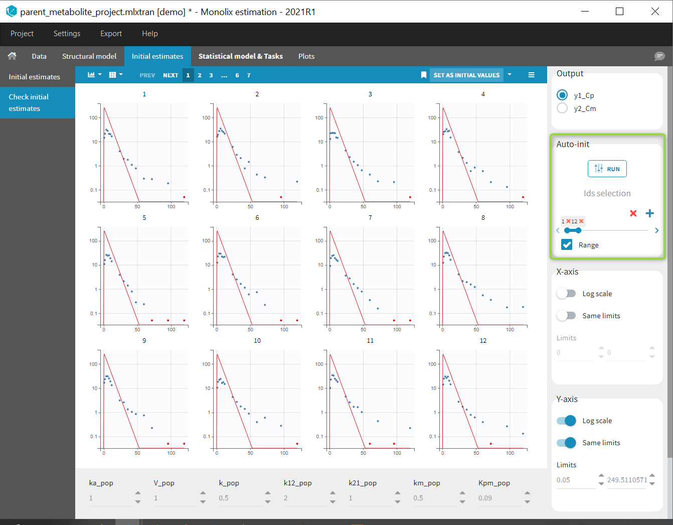
By clicking on RUN, Monolix will compute initial population parameters that best fit the data points, starting from parameter values currently used in the initial estimates panel, and using the data from the 12 first individuals by default, and from all observations mapped to a model output. It is possible to change the set of individuals used in the Ids selection panel just below the RUN button.
The computation is done with a custom optimization method, on the pooled data, without inter-individual variability. The purpose is not to find a perfect match but rather to have all the parameters in the good range for starting the population modeling approach. While auto-init is running, we show the evolution of the cost of the optimization algorithm over the iterations. It is possible to stop the algorithm at any time if you find the cost has decreased sufficiently and you want to have a look at the parameter values. Note that the more individuals are selected, the longer the run will take. Moreover, it may be easier for the auto-init algorithm to find a point in the parameter space that is sensitive to specific model features (eg a third compartment, a complex absorption) if you select only a few individuals (1-3 for instance) for which this feature can be observed.
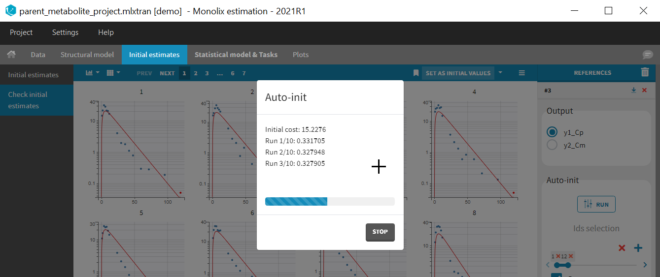
After clicking on the button, the population parameters are updated and the corresponding fit is displayed. To use these parameters as initial estimates, you need to click on the button “SET AS INITIAL VALUES”. A new reference appears with previous parameter values so that you can come back to previous values if you are not satisfied with the fit.
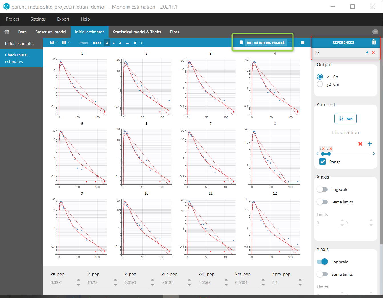
Note that the auto-init procedure takes into account the current initial values. Therefore, in the few cases where the auto-init might give poor results, it is possible to improve the results by changing manually the parameter values before running the auto-init again.
5.1.2.Population parameter estimation using SAEM
- Purpose
- Calculations: the SAEM algorithm
- Running the population parameter estimation task
- Outputs
- In the graphical user interface
- In the output folder
- Settings
- Good practices, troubleshooting and tips
Purpose
The estimation of the population parameters is the key task in non-linear mixed effect modeling. In Monolix, it is performed using the Stochastic Approximation Expectation-Maximization (SAEM) algorithm [1]. SAEM has been shown to be extremely efficient for both simple and a wide variety of complex models: categorical data [2], count data [3], time-to-event data [4], mixture models [5–6], differential equation based models, censored data [7], … The convergence of SAEM has been rigorously proven [1] and its implementation in Monolix is particularly efficient. No other algorithms are available in Monolix.
Calculations: the SAEM algorithm
Running the population parameter estimation task
Overview
The pop-up window which permits to follow the progress of the task is shown below. The algorithm starts with a small number (5 by default) of burn-in iterations for initialization which are displayed in the following way: (note that this step can be so fast that it is not visible by the user)
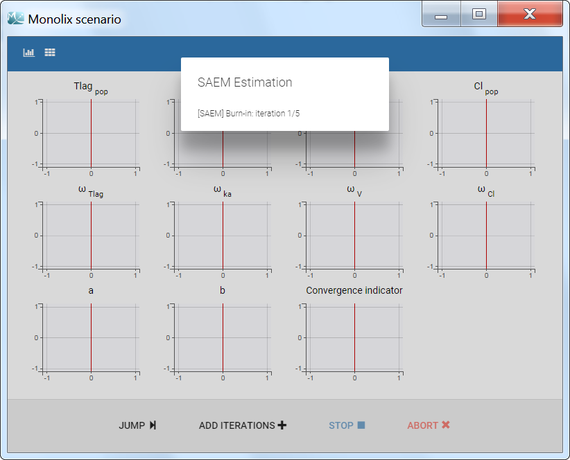
Afterwards, the evolution of the value for each population parameter over the iterations of the algorithm is displayed. The red line marks the switch from the exploratory phase to the smoothing phase. The exact value at each iterations can be followed by hovering over the curve (as for Cl_pop below). The convergence indicator (in purple) helps to detect that convergence has been reached (see below for more details).

Dependencies between tasks
The “Population parameter” estimation task must be launched before running any other task. To skip this task, the user can fix all population parameters. If all population parameters have been set to “fixed”, the estimation will stop after a single iteration and allow the user to continue with the other tasks.
The convergence indicator
The convergence indicator (also sometimes called complete likelihood) is defined as the joint probability distribution of the data and the individual parameters and can be decomposed using Bayes law:
\(\sum_{i=1}^{N_{\text{ind}}}\log\left(p(y_i, \phi_i; \theta)\right)=p(y_i| \psi_i; \theta)p(\psi_i; \theta)\)
Those two terms have an analytical expression and are easy to calculate, using as \(\phi_i\) the individual parameters drawn by MCMC for the current iteration of SAEM. This quantity is calculated at each SAEM step and is useful to assess the convergence of the SAEM algorithm.
The convergence indicator aggregates the information from all parameters and can serve to detect if the SAEM algorithm has already converged or not. When the indicator is stable, that is it oscillates around the same value without drifting, then we can be pretty confident that the maximum likelihood has been achieved. The convergence indicator is used, among other measures, in the auto-stop criteria to switch from the exploratory phase to the smoothing phase.
Note that the likelihood (i.e the objective function) \(\sum_{i=1}^{N_{\text{ind}}}\log\left(p(y_i; \theta)\right)\) cannot be computed in closed form because the individual parameters \(\phi_i\) are unobserved. It requires to integrate over all possible values of the individual parameters. Thus, to estimate the log-likelihood an importance sampling Monte Carlo method is used in a separate task (or an approximation is calculated via linearization of the model).
The simulated annealing
The simulated annealing option (setting enabled by default) permits to keep the explored parameter space large for a longer time (compared to without simulated annealing). This allows to escape local maximums and improve the convergence towards the global maximum.
In practice, the simulated annealing option constrains the variance of the random effects and the residual error parameters to decrease by maximum 5% (by default – the setting “Decreasing rate” can be changed) from one iteration to the next one. As a consequence, the variances decrease more slowly:
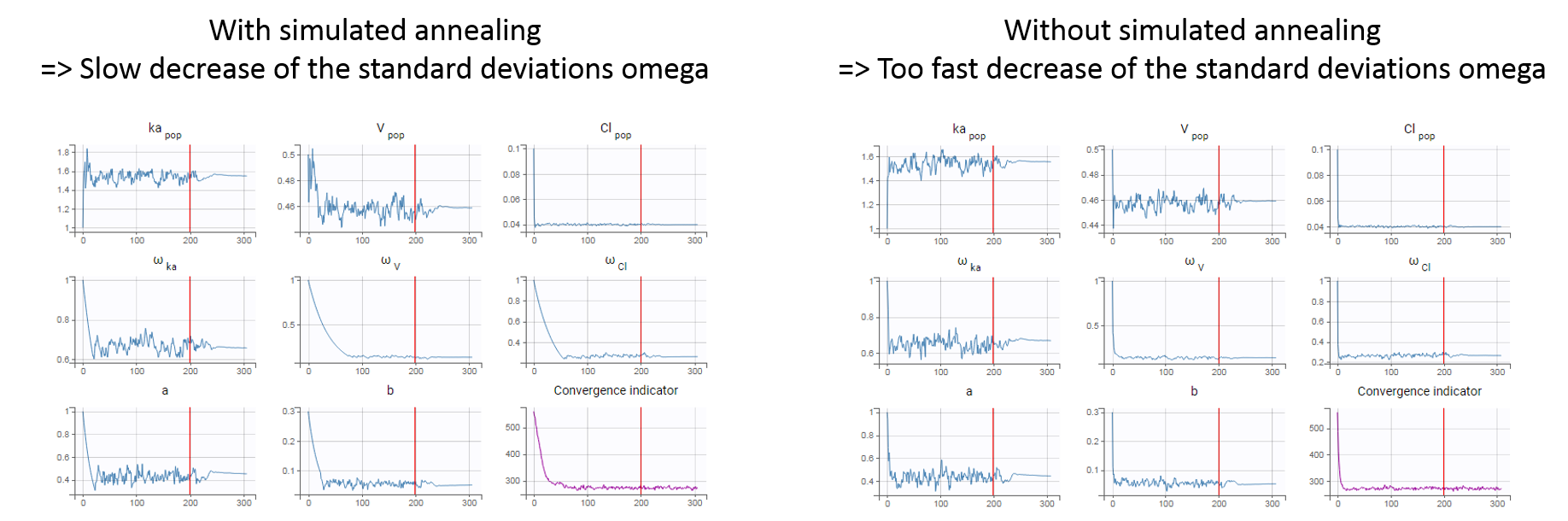
The size of the parameter space explored by the SAEM algorithm depends on individual parameters sampled from their conditional distribution via Markov Chain Monte Carlo. If the standard deviation of the conditional distributions is large, the individual parameters sampled at iteration k can be quite far away from those at iteration (k-1), meaning a large exploration of the parameter space. The standard deviation of the conditional distribution depends on the standard deviation of the random effects (population parameters ‘omega’). Indeed, the conditional distribution is \(p(\psi_i|y_i;\hat{\theta})\) with \(\psi_i\) the individual parameters for individual \(i\), \(\hat{\theta}\) the estimated population parameters, and \(y_i\) the data (observations) for individual \(i\). The conditional distribution thus depends on the population parameters, and the larger the population parameters ‘omega’, the larger the standard deviation of the conditional distribution. That’s why we want to keep large ‘omega’ values during the first iterations.
Methods for the parameters without variability
Parameters without variability are not estimated in the same way as parameters with variability. Indeed, the SAEM algorithm requires to draw parameter values from their marginal distribution, which exists only for parameters with variability.
Several methods can be used to estimate the parameters without variability. By default, these parameters are optimized using the Nelder-Mead simplex algorithm (Matlab’s fminsearch method). Other options are also available in the SAEM settings:
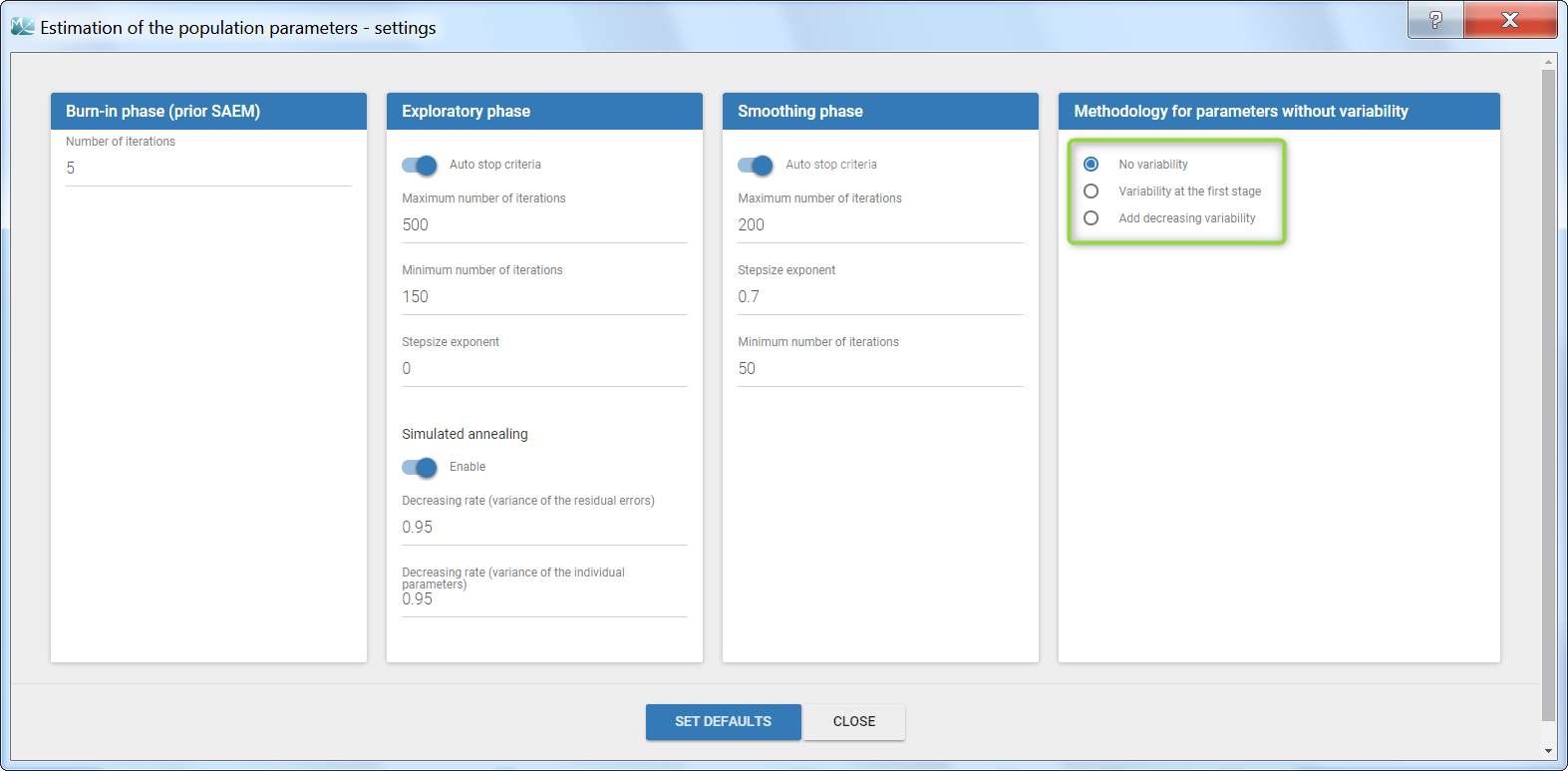
- No variability (default): optimization via Nelder-Mead simplex algorithm
- Add decreasing variability: an artificial variability (i.e random effects) is added for these parameters, allowing estimation via SAEM. The variability starts at omega=1 and is progressively decreased such that at the end of the estimation process, the parameter has a variability of 1e-5. The decrease in variability is exponential with a rate based on the maximum number of iterations for both the exploratory and smoothing phases. Note that if the autostop is triggered, the resulting variability might me higher.
- Variability at the first stage: during the exploratory phase of SAEM, an artificial variability is added and progressively forced to 1e-5 (same as above). In the smoothing phase, the Nelder-Mead simplex algorithm is used.
Depending on the specific project, one or the other method may lead to a better convergence. If the default method does not provide satisfying results, it is worth trying the other methods. In terms of computing time, if all parameters are without variability, the first option will be faster because only the Nelder-Mead simplex algorithm will be used to estimate all the fixed effects. If some parameters have random effects, the first option will be slower because the Nelder-Mead and the SAEM algorithm are computed at each step. In that case the second or third option will be faster because only the SAEM algorithm will be required when the artificial variability is added.
Alternatively, the standard deviation of the random effects can be fixed to a small value, for instance 5% for log-normally distributed parameters. (See next section on how to enforce a fixed value). With this method, the SAEM algorithm can be used, and the variability is kept small.
Other estimation methods: fixing population parameters or Bayesian estimation
Instead of the default estimation method with SAEM, it is possible to fix a population parameter, or set a prior on the estimate and use Bayesian estimation. This page gives details on these methods and how to use them.
Outputs
In the graphical user interface
The estimated population parameters are displayed in the POP.PARAM section of the RESULTS tab. Fixed effects names are “*_pop”, the standard deviation of the random effects “omega_*”, parameters of the error model “a”, “b”, “c”, the correlation between random effects “corr_*_*” and parameters associated to covariates “beta_*_*”. The standard deviation of the random effects is also expressed as coefficient of variation (CV) – a feature present in versions Monolix 2023 or above. The CV calculation depends on the parameter distribution:
- lognormal: \(CV=100*\sqrt{exp(\omega_p^2) -1}\)
- normal: \(CV=100*\frac{\omega_p}{p_{pop}}\)
- logitnormal and probitnormal: the CV is computed by Monte-Carlo. 100000 samples X are drawn from the distribution (defined by \(\omega_p\) and \(p_{pop}\)) and the CV is calculated as the ratio of the sample standard deviation over the sample mean: \(CV=100*\frac{sd(X)}{mean(X)}\)
When you run the “Standard errors” task, then the population parameter table contains also the standard error (s.e) and relative standard error (r.s.e). Note that the CV% represents the inter-individual variability, while the RSE% represents the uncertainty on the estimated parameters.
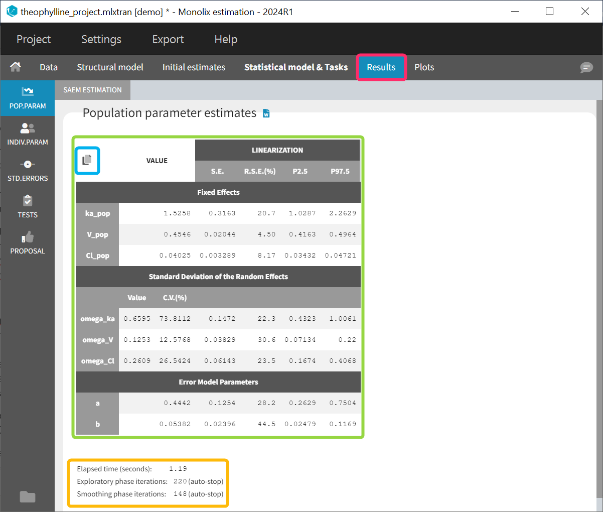
Starting from version 2024, alongside the standard errors, the upper and lower percentiles, here P2.5 and P97.5 of the confidence interval with level 1−\( \alpha\) are computed for population parameters. This calculation depends on the execution of the “Standard errors” task, as it relies on the standard error of the respective parameter. In order to take into account the boundaries of the parameters (e.g omega or V_pop cannot be negative), the SE is transformed into the gaussian domain, the CI in gaussian domain is calculated assuming a normal distribution and finally the CI is backtransformed. Its transformation is determined by the type of parameter and its distribution assumption:
- Normal distributed parameters: \(CI_{1-\alpha} (\theta _{pop})=[\theta_{pop} + q_{\alpha /2}\times s.e.(\theta_{pop}), ~\theta_{pop} + q_{1 – \alpha /2}\times s.e.(\theta_{pop})]\). This applies for typical values (fixed effects) of normally distributed parameters and covariate effects (betas).
- Lognormal distributed parameters: \(CI_{1-\alpha} (\theta _{pop})=[\exp(\mu_{pop} + q_{\alpha /2}\times s.e.(\mu_{pop})), ~\exp(\mu_{pop} + q_{1 – \alpha /2}\times s.e.(\mu_{pop}))]\), where \( \mu_{pop} = \ln(\theta_{pop})\). This applies to typical values (fixed effects) of lognormally distributed parameters, standard deviations of the random effects (omegas), and error model parameters.
- Logitnormal distributed parameters: \(CI_{1-\alpha} (\theta _{pop})=[logit^{-1}(\mu_{pop} + q_{\alpha /2}\times s.e.(\mu_{pop})), ~logit^{-1}(\mu_{pop} + q_{1 – \alpha /2}\times s.e.(\mu_{pop}))]\), where \( \mu_{pop} = logit(\theta_{pop})\). This applies to typical values (fixed effects) of logit-normally distributed parameters and correlation parameters.
where \(q_{\alpha /2}\) is the quantile of order \( \alpha /2\) for a standard normal distribution. The confidence interval level \( \alpha\) can be modified in the settings of the “Standard errors” task within the Statistical Model & Tasks tab by clicking on the wrench icon.
Information about the SAEM task performance are below the table (orange frame):
- The total elapsed time for this task
- The number of iterations in the exploratory and smoothing phases, along with a message that indicates whether the convergence has been reached (“auto-stop”), or if the algorithm arrived at the maximum number of iterations (“stopped at the maximum number of iterations/auto-stop criteria have not been reached”) or if it was stopped by the user (“manual stop”). (for Monolix versions 2021 or above)
A “Copy table” icon on the top of the table allows to copy it in Excel, Word, etc. The table format and display is kept.
Starting from version 2024R1, if categorical covariate effects are included in the statistical model, a “Display fixed effects by category” toggle allows to add a section named “Fixed effects by category” in the table, with the values of the typical population parameters in each category of the categorical covariates and their SEs, RSEs and confidence intervals.
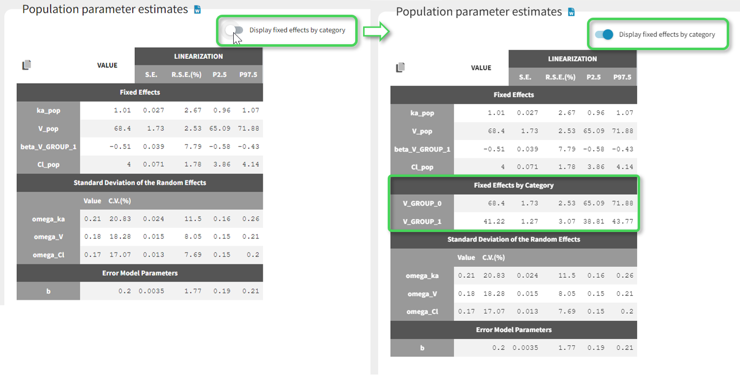
In the output folder
After having run the estimation of the population parameters, the following files are available:
- summary.txt: contains the estimated population parameters (and the number of iterations in Monolix2021R1), in a format easily readable by a human (but not easy to parse for a computer)
- populationParameters.txt: contains the estimated population parameters (by default in csv format), including the CV.
- populationParametersByGroups.txt: contains the estimated population parameters by categories of categorical covariates included in the statistical model. This file is not generated if there are no categorical covariate effects.
- predictions.txt: contains for each individual and each observation time, the observed data (y), the prediction using the population parameters and population median covariates value from the data set (popPred_medianCOV), the prediction using the population parameters and individual covariates value (popPred), the prediction using the individual approximate conditional mean calculated from the last iterations of SAEM (indivPred_SAEM) and the corresponding weighted residual (indWRes_SAEM).
- IndividualParameters/estimatedIndividualParameters.txt: individual parameters corresponding to the approximate conditional mean, calculated as the average of the individual parameters sampled by MCMC during all iterations of the smoothing phase. When several chains are used (see project settings), the average is also done over all chains. Values are indicated as *_SAEM in the file.
Parameters without variability:- method “no variability” or “variability at the first stage”: *_SAEM represents the value at the last SAEM iteration, so the estimated population parameter plus the covariate effects. In absence of covariate, all individuals have the same value.
- method “add decreasing variability”: *_SAEM represents the average of all iterations of the smoothing phase. This value can be slightly different from individual to individual, even in te absence of covariates.
- IndividualParameters/estimatedRandomEffects.txt: individual random effects corresponding to the approximate conditional mean, calculated using the last estimations of SAEM (*_SAEM).
For parameters without variability, see above.
More details about the content of the output files can be found here.
Settings
The settings are accessible through the interface via the button next to the parameter estimation task.
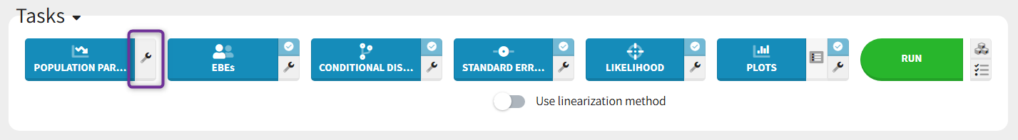
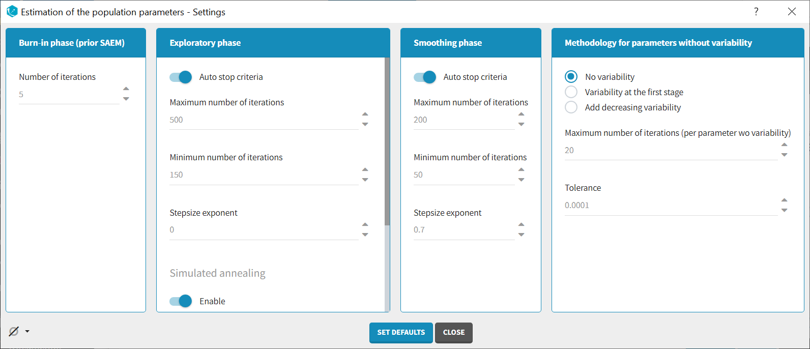
Burn-in phase:
The burn-in phase corresponds to an initialization of SAEM: individual parameters are sampled from their conditional distribution using MCMC using the initial values for the population parameters (no update of the population parameter estimates).
Note: the meaning of the burn-in phase in Monolix is different to what is called burn-in in Nonmem algorithms.
- Number of iterations (default: 5): number of iterations of the burn-in phase
Exploratory phase:
- Auto-stop criteria (default: yes): if ticked, auto-stop criteria are used to automatically detect convergence during the exploratory phase. If convergence is detected, the algorithm switches to the smoothing phase before the maximum number of iterations. The criteria take into account the stability of the convergence indicator, omega parameters and error model parameters.
- Maximum number of iterations (default: 500, if auto-stop ticked): maximum number of iterations for the exploratory phase. Even if the auto-stop criteria are not fulfilled, the algorithm switches to the smoothing phase after this maximum number of iterations. A warning message will be displayed in the GUI if the maximum number of iterations is reached while the auto-stop criteria are not fulfilled.
- Minimum number of iterations (default: 150, if auto-stop ticked): minimum number of iterations for the exploratory phase. This value also corresponds to the interval length over which the auto-stop criteria are tested. A larger minimum number of iterations means that the auto-stop criteria are harder to reach.
- Number of iterations (default: 500, if auto-stop unticked): fixed number of iterations for the exploratory phase.
- Step-size exponent (default: 0): The value, comprised between 0 and 1, represents memory of the stochastic process, i.e how much weight is given at iteration k to the value of the previous iteration compared to the new information collected. A value 0 means no memory, i.e the parameter value at iteration k is built based on the information collected at that iteration only, and does not take into account the value of the parameter at the previous iteration.
- Simulated annealing (default: enabled): the Simulated Annealing version of SAEM permits to better explore the parameter space by constraining the standard deviation of the random effects to decrease slowly.
- Decreasing rate for the variance of the residual errors (default: 0.95, if simulated annealing enabled): the residual error variance (parameter “a” for a constant error model for instance) at iteration k is constrained to be larger than the decreasing rate times the variance at the previous iteration.
- Decreasing rate for the variance of the individual parameters (default: 0.95, if simulated annealing enabled): the variance of the random effects at iteration k is constrained to be larger than the decreasing rate times the variance at the previous iteration.
Smoothing phase:
- Auto-stop criteria (default: yes): if ticked, auto-stop criteria are used to automatically detect convergence during the smoothing phase. If convergence is detected, the algorithm stops before the maximum number of iterations.
- Maximum number of iterations (default: 200, if auto-stop ticked): maximum number of iterations for the smoothing phase. Even if the auto-stop criteria are not fulfilled, the algorithm stops after this maximum number of iterations.
- Minimum number of iterations (default: 50, if auto-stop ticked): minimum number of iterations for the smoothing phase. This value also corresponds to the interval length over which the auto-stop criteria is tested. A larger minimum number of iterations means that the auto-stop criteria is harder to reach.
- Number of iterations (default: 200, if auto-stop unticked): fixed number of iterations for the smoothing phase.
- Step-size exponent (default: 0.7): The value, comprised between 0 and 1, represents memory of the stochastic process, i.e how much weight is given at iteration k to the value of the previous iteration compared to the new information collected. The value must be strictly larger than 0.5 for the smoothing phase to converge. Large values (close to 1) will result in a smoother parameter trajectory during the smoothing phase, but may take longer to converge to the maximum likelihood estimate.
Methodology for parameters without variability (if parameters without variability are present in the model):
The SAEM algorithm requires to draw parameter values from their marginal distribution, which does not exist for parameters without variability. These parameters are thus estimated via another method, which can be chosen among:
- No variability (default choice): After each SAEM iteration, the parameter without variability are optimized using the Nelder-Mead simplex algorithm. The absolute tolerance (stopping criteria) is 1e-4 and the maximum number of iterations 20 times the number of parameters to calculate via this algorithm.
- Add decreasing variability: an artificial variability is added for these parameters, allowing estimation via SAEM. The variability is progressively decreased such that at the end of the estimation process, the parameter has a variability of 1e-5.
- Variability in the first stage: during the exploratory phase, an artificial variability is added and progressively forced to 1e-5 (same as above). In the smoothing phase, the Nelder-Mead simplex optimization algorithm is used.
Handling parameters without variability is also discussed here.
Set all SAEM iterations to zero in one click
The icon on the bottom left provides a shortcut to set all SAEM iterations to zero (in all three phases). This is convenient if the user wish to skip the estimation of the population parameters and keep the initial estimates as population estimates to run the other tasks, since running SAEM first is mandatory. It is not equivalent to fixing all population parameters, since standard errors are not estimated for fixed parameters, while they will be estimated for the initial estimates in this case. The action can be easily reversed with the second shortcut to reset default SAEM iterations.
Good practice, troubleshooting and tips
Choosing to enable or disable the simulated annealing
As the simulated annealing option permits to more surely find the global maximum, it should be used during the first runs, when the initial values may be quite far from the final estimates.
On the other side, the simulated annealing option may keep the omega values artificially high, even after a large number of SAEM iterations. This may prevent the identification of parameters for which the variability is in fact zero and lead to NaN in the standard errors. So once good initial values have been found and there is no risk to fall in a local maximum, the simulated annealing option can be disabled. Below we show an example where removing the simulated annealing permits to identify parameters for which the inter-individual variability can be removed.
Example: The dataset used in the tobramycin case study is quite sparse. In these conditions, we expect that estimating the inter-individual variability for all parameters will be difficult. In this case, the estimation can be done in two steps, as shown below for a two-compartments model on this dataset:
- First, we run SAEM with the simulated annealing option (default setting), which facilitates the convergence towards the global maximum. All four parameters V, k, k12 and k21 have random effects. The estimated parameters are shown below:
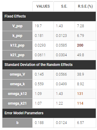
The parameters omega_k12 and omega_k21 have high standard errors, suggesting that the variability is difficult to estimate. The omega_k12 and omega_k21 values themselves are also high (100% inter-individual variability), suggesting that they may have been kept too high due to the simulated annealing.
- As a second step, we use the last estimates as new initial values (as shown here), and run SAEM again after disabling the simulated annealing option. On the plot showing the convergence of SAEM, we can see omega_V, omega_k12 and omega_k21 decreasing to very low values. The data is too sparse to correctly identify the inter-individual variability for V, k12 and k21. Thus, their random effects can be removed, but the random effect of k can be kept.
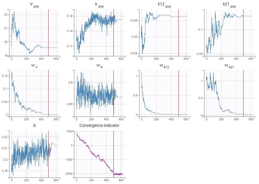
Note that because the omega_V, omega_k12 and omega_k21 parameters decrease without stabilizing, the convergence indicator does the same.
5.1.2.1.The convergence indicator
When you launch the estimation of the population parameters, you can see the evolution of the population parameter estimates over the iterations of the SAEM algorithm but also the convergence indicator in purple.

The convergence indicator is the complete log-likelihood. It can help to follow convergence.
Note that the complete likelihood is not the same as the log-likelihood computed as separate task.
Log-likelihood
The likelihood is the probability density of the data given the population parameter, so the log-likelihood is defined as:
\(\sum_{i=1}^{N_{\text{ind}}}\log\left(p(y_i; \theta)\right)\)
The likelihood is the objective function, therefore it is the relevant quantity to compare model, but unfortunately it cannot be computed in closed form because the individual parameters \(\phi_i\) are unobserved. It requires to integrate over all possible values of the individual parameters. Thus, to estimate the log-likelihood an importance sampling Monte Carlo method is used in a separate task (or an approximation is calculated via linearization of the model).
Complete log-likelihood
On the contrary, the complete likelihood refers to the joint probability distribution of the data and the individual parameters. The convergence indicator (complete log-likelihood) is then defined as:
\(\sum_{i=1}^{N_{\text{ind}}}\log\left(p(y_i, \phi_i; \theta)\right)\)
The joint probability distribution can be decomposed using Bayes law as:
\(p(y_i, \psi_i; \theta)=p(y_i| \psi_i; \theta)p(\psi_i; \theta)\)
Those two terms have an analytical expression and are easy to calculate, using as \(\phi_i\) the individual parameters drawn by MCMC for the current iteration of SAEM. This quantity is calculated at each SAEM step and is useful to assess the convergence of the SAEM algorithm.
Typical shape of the convergence indicator
Typically, the convergence indicator decreases progressively and then stabilizes. The convergence indicator aggregates the information from all parameters and can serve to detect if the SAEM algorithm has already converged or not. When the indicator is stable, that is it oscillates around the same value without drifting, then we can be pretty confident that the maximum likelihood has been achieved.
5.1.2.2.Simulated annealing
The estimation of the population parameters with SAEM includes a method of simulated annealing. It is possible to disable this option in the settings of SAEM. The option is enabled by default.
Purpose
The simulated annealing option permits to keep the explored parameter space large for a longer time (compared to without simulated annealing). This allows to escape local maximums and improve the convergence towards the global maximum.
Calculations
In practice, the simulated annealing option constrains the variance of the random effects and the residual error parameters to decrease by maximum 5% (by default, the setting “Decreasing rate” can be changed) from one iteration to the next one. As a consequence, the variances decrease more slowly:
The size of the parameter space explored by SAEM depends on individual parameters sampled from their conditional distribution via Markov Chain Monte Carlo. If the standard deviation of the conditional distributions is large, the individual parameters sampled at iteration k can be quite far away from those at iteration (k-1), meaning a large exploration of the parameter space. The standard deviation of the conditional distribution depends on the standard deviation of the random effects (population parameters ‘omega’). Indeed, the conditional distribution is \(p(\psi_i|y_i;\hat{\theta})\) with \(\psi_i\) the individual parameters for individual \(i\), \(\hat{\theta}\) the estimated population parameters, and \(y_i\) the data (observations) for individual \(i\). The conditional distribution thus depends on the population parameters, and the larger the population parameters ‘omega’, the larger the standard deviation of the conditional distribution. That’s why we want to keep large ‘omega’ values during the first iterations.
Settings
The simulated annealing option can be disabled or enabled in the “Population parameters” task settings. In addition, the settings allow to change the default decreasing rates for the standard deviations of the random effects and the residual errors.
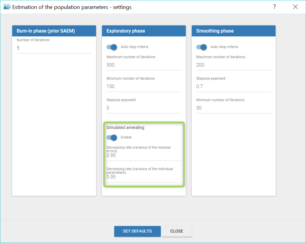
Choosing to enable or disable the simulated annealing
As the simulated annealing option permits to more surely find the global maximum, it should be used during the first runs, when the initial values may be quite far from the final estimates.
On the other side, the simulated annealing option may keep the omega values artificially high, even after a large number of SAEM iterations. This may prevent the identification of parameters for which the variability is in fact zero and lead to NaN in the standard errors. So once good initial values have been found and there is no risk to fall in a local maximum, the simulated annealing option can be disabled. Below we show an example where removing the simulated annealing permits to identify parameters for which the inter-individual variability can be removed.
Example: identifying parameters with no variability
The dataset used in the tobramycin case study is quite sparse. In these conditions, we expect that estimating the inter-individual variability for all parameters will be difficult. In this case, the estimation can be done in two steps, as shown below for a two-compartments model on this dataset:
- First, we run SAEM with the simulated annealing option (default setting), which facilitates the convergence towards the global maximum. All four parameters V, k, k12 and k21 have random effects. The estimated parameters are shown below:
The parameters omega_k12 and omega_k21 have high standard errors, suggesting that the variability is difficult to estimate. The omega_k12 and omega_k21 values themselves are also high (100% inter-individual variability), suggesting that they may have been kept too high due to the simulated annealing.
- As a second step, we use the last estimates as new initial values (as shown here), and run SAEM again after disabling the simulated annealing option. On the plot showing the convergence of SAEM, we can see omega_V, omega_k12 and omega_k21 decreasing to very low values. The data is then too sparse to correctly identify the inter-individual variability for V, k12 and k21. Thus, their random effects can be removed, but the random effect of k can be kept.
Note that because the omega_V, omega_k12 and omega_k21 parameters decrease without stabilizing, the convergence indicator does the same.
5.1.2.3.Bayesian estimation
In the tab “Initial estimates”, clicking on the wheel icon next to a population parameters opens a window to choose among three estimation methods (see image below). “Maximum Likelihood Estimation” corresponds to the default method using SAEM, detailed on this page. “Maximum A Posteriori Estimation” corresponds to Bayesian estimation, and “Fixed” to a fixed parameter.
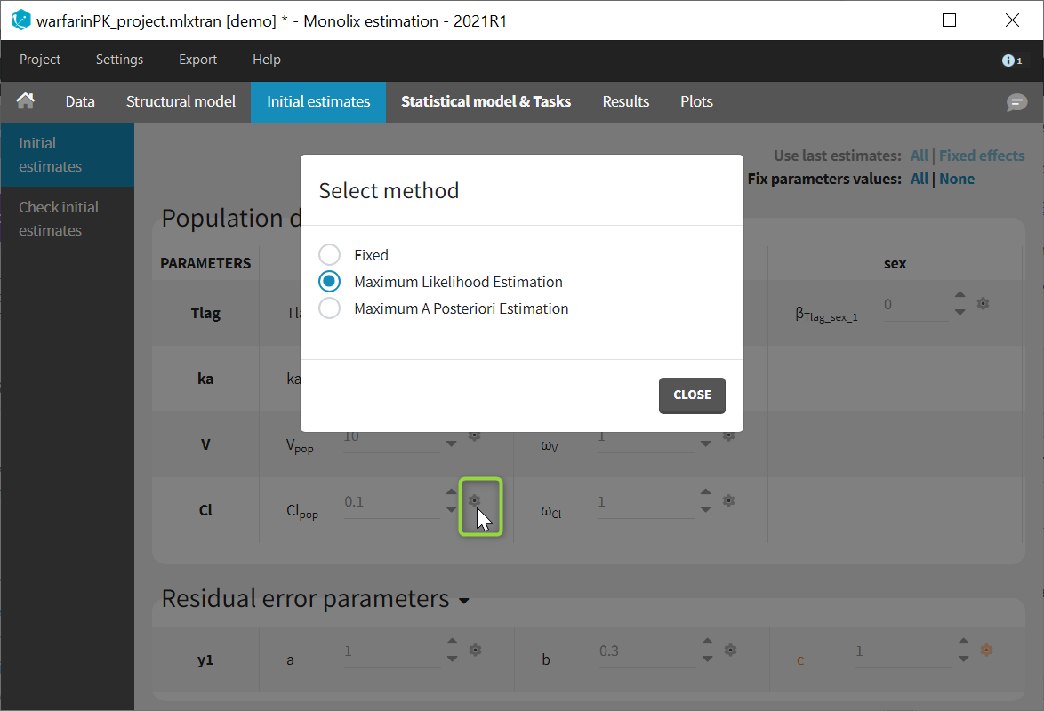
Bayesian estimation
Purpose
Bayesian estimation allows to take into account prior information in the estimation of parameters. It is called in Monolix Maximum A Posteriori estimation, and it corresponds to a penalized maximum likelihood estimation, based on a prior distribution defined for a parameter. The weight of the prior in the estimation is given by the standard deviation of the prior distribution.
Objectives: learn how to combine maximum likelihood estimation and Bayesian estimation of the population parameters.
Projects: theobayes1_project, theobayes2_project,
Introduction
The Bayesian approach considers the vector of population parameters \(\theta\) as a random vector with a prior distribution \(\pi_\theta\). We can then define the *posterior distribution* of \(\theta\):
\(\begin{aligned} p(\theta | y ) &= \frac{\pi_\theta( \theta )p(y | \theta )}{p(y)} \\ &= \frac{\pi_\theta( \theta ) \int p(y,\psi |\theta) \, d \psi}{p(y)} . \end{aligned} \)
We can estimate this conditional distribution and derive statistics (posterior mean, standard deviation, quantiles, etc.) and the so-called maximum a posteriori (MAP) estimate of \(\theta\):
\(\begin{aligned} \hat{\theta}^{\rm MAP} &=\text{arg~max}_{\theta} p(\theta | y ) \\ &=\text{arg~max}_{\theta} \left\{ {\cal LL}_y(\theta) + \log( \pi_\theta( \theta ) ) \right\} . \end{aligned} \)
The MAP estimate maximizes a penalized version of the observed likelihood. In other words, MAP estimation is the same as penalized maximum likelihood estimation. Suppose for instance that \(\theta\) is a scalar parameter and the prior is a normal distribution with mean \(\theta_0\) and variance \(\gamma^2\). Then, the MAP estimate is the solution of the following minimization problem:
\(\hat{\theta}^{\rm MAP} =\text{arg~min}_{\theta} \left\{ -2{\cal LL}_y(\theta) + \frac{1}{\gamma^2}(\theta – \theta_0)^2 \right\} .\)
This is a trade-off between the MLE which minimizes the deviance, \(-2{\cal LL}_y(\theta)\), and \(\theta_0\) which minimizes \((\theta – \theta_0)^2\). The weight given to the prior directly depends on the variance of the prior distribution: the smaller \(\gamma^2\) is, the closer to \(\theta_0\) the MAP is. In the limiting case, \(\gamma^2=0\); this means that \(\theta\) is fixed at \(\theta_0\) and no longer needs to be estimated. Both the Bayesian and frequentist approaches have their supporters and detractors. But rather than being dogmatic and following the same rule-book every time, we need to be pragmatic and ask the right methodological questions when confronted with a new problem.
All things considered, the problem comes down to knowing whether the data contains sufficient information to answer a given question, and whether some other information may be available to help answer it. This is the essence of the art of modeling: find the right compromise between the confidence we have in the data and our prior knowledge of the problem. Each problem is different and requires a specific approach. For instance, if all the patients in a clinical trial have essentially the same weight, it is pointless to estimate a relationship between weight and the model’s PK parameters using the trial data. A modeler would be better served trying to use prior information based on physiological knowledge rather than just some statistical criterion.
Generally speaking, if prior information is available it should be used, on the condition of course that it is relevant. For continuous data for example, what does putting a prior on the residual error model’s parameters mean in reality? A reasoned statistical approach consists of including prior information only for certain parameters (those for which we have real prior information) and having confidence in the data for the others. Monolix allows this hybrid approach which reconciles the Bayesian and frequentist approaches. A given parameter can be
- a fixed constant if we have absolute confidence in its value or the data does not allow it to be estimated, essentially due to lack of identifiability.
- estimated by maximum likelihood, either because we have great confidence in the data or no information on the parameter.
- estimated by introducing a prior and calculating the MAP estimate or estimating the posterior distribution.
Computing the Maximum a posteriori (MAP) estimate
- demo project: theobayes1_project (data = ‘theophylline_data.txt’ , model = ‘lib:oral1_1cpt_kaVCl.txt’)
We want to introduce a prior distribution for \(ka_{\rm pop}\) in this example. Click on the option button

and select Maximum A Poteriori Estimation

We propose a typical value, here 2 and standard deviation 0.1 for \(ka_{\rm pop}\) and to compute the MAP estimate for \(ka_{\rm pop}\). The parameter is then colored in purple.

Starting from the 2021 version, it is possible to select maximum a posteriori estimation also for the omega parameters (standard deviations of the random effects). In this case, an inverse Wishart is set as a prior distribution for the omega matrix.
The following distributions for the priors are used:
- typical value (*_pop): the distribution of the prior is the same as the distribution of the parameter. For instance, if ka has been set with a lognormal distribution in the “Statistical model & Tasks” tab, a lognormal distribution is also used for the prior on ka_pop. When a lognormal distribution is used, setting sd=0.1 roughtly corresponds to 10% uncertainty in the provided prior value for ka_pop.
- covariate effects (beta_*): a normal distribution is used, to allow betas to be either positive or negative.
- standard deviations (omega_*) [starting version 2021]: an inverse Wishart distribution is used. Inverse Wisharts are common prior distributions for variance-covariance matrices as they allow to fulfill the positive-definite matrix requirement. The weight of the prior in the estimation is based on the number of degrees of freedom (df) of the inverse Wishart, instead of a standard deviation. More degrees of freedom correspond to a higher constrain of the prior in the omega estimation. In Monolix, each omega parameter is handled as a 1×1 matrix with its own degree of freedom, independently from the other omegas. The univariate inverse Wishart \( W^{-1}(df, (df+2)\omega_{typ}) \) simplifies to an inverse gamma distribution with shape parameter \(\alpha=df/2 \) and scale parameter \(\beta=\omega_{typ}*(df+2)/2\). The coefficient of variation is thus \(CV=\frac{1}{\sqrt{\frac{df}{2}-2}}\). To obtain a 20% uncertainty on omega (CV=0.2), the user can set df=50.
- correlations: it is currently not possible to set a prior on the correlation parameters
It is common to set the initial value of the parameter to be the same as the typical value of the prior. Note that the default value for the typical value of the prior is set to the initial value of the parameter. However, if the initial value of the parameter is modified afterwards, the typical value of the prior is not updated automatically.
Fixing the value of a parameter
Population parameters can be fixed to their initial values, in this case they are not estimated. It is possible to fix one, several or all population parameters, among the fixed effects, standard deviations of random effects, and error model parameters. In Monolix2021, it is also possible to fix correlation parameters.
To fix a population parameter, click on the wheel next to the parameter in the tab “Initial estimates” and select “Fixed”, like on the image below:
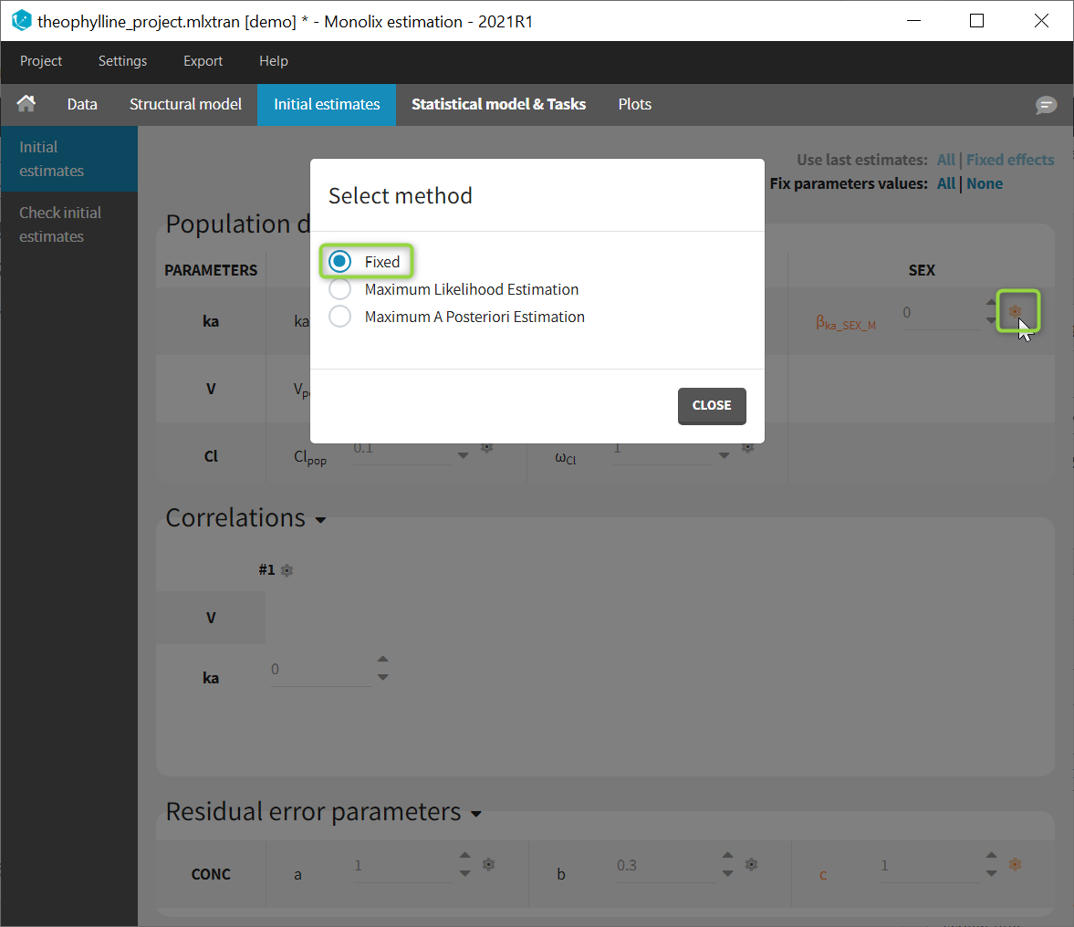
Fixed parameters appear on this tab in red. In Monolix2021, they are also colored in red in the subtab “Check initial estimates”.
- theobayes2_project (data = ‘theophylline_data.txt’ , model = ‘lib:oral1_1cpt_kaVCl.txt’)
We can combine different strategies for the population parameters: Bayesian estimation for \(ka_{\rm pop}\), fixed value for \(V_{\rm pop}\) and maximum likelihood estimation for \(Cl_{\rm pop}\), for instance.

Remark:
- The parameter \(V_{\rm pop}\) is fixed and then colored in red.
- \(V_{\rm pop}\) is not estimated (it’s s.e. is not computed) but the standard deviation \(\omega_{V}\) is estimated as usual.
5.1.3.EBEs
- Purpose
- Calculation of the EBEs (conditional mode)
- Conditional distribution
- Mode of the conditional distribution
- Individual random effects
- Algorithm
- Running the EBEs task
- Outputs
- In the graphical user interface
- In the output folder
- Settings
- Calculate EBEs for a new data set using an existing model
Purpose
EBEs stands for Empirical Bayes Estimates. The EBEs are the most probable value of the individual parameters (parameters for each individual), given the estimated population parameters and the data of each individual. In a more mathematical language, they are the mode of the conditional parameter distribution for each individual.
These values are useful to compute the most probable prediction for each individual, for comparison with the data (for instance in the Individual Fits plot).
Calculation of the EBEs (conditional mode)
When launching the “EBEs” task, the mode of the conditional parameter distribution is calculated.
Conditional distribution
The conditional distribution is \( p(\psi_i|y_i;\hat{\theta})\) with \(\psi_i\) the individual parameters for individual i, \(\hat{\theta}\) the estimated population parameters, and \(y_i\) the data (observations) for individual i. The conditional distribution represents the uncertainty of the individual’s parameter value, taking into account the information at hand for this individual: the observed data for that individual, the covariate values for that individual and the fact that the individual belongs to the population for which we have already estimated the typical parameter value (fixed effects) and the variability (standard deviation of the random effects). It is not possible to directly calculate the probability for a given \(\psi_i\) (no closed form), but is possible to obtain samples from the distribution using a Markov-Chain Monte-Carlo procedure (MCMC). This is detailed more on the Conditional Distribution page.
Mode of the conditional distribution
The mode is the parameter value with the highest probability:
$$ \hat{\psi}_i^{mode} = \underset{\psi_i}{\textrm{arg max }}p(\psi_i|y_i;\hat{\theta})$$
To find the mode, we thus need to maximize the conditional probability with respect to the individual parameter value \(\psi_i\).
Individual random effects
Once the individual parameters values \(\psi_i\) are known, the corresponding individual random effects can be calculated using the population parameters and covariates. Taking the example of a parameter \(\psi\) having a normal distribution within the population and that depends on the covariate \(c\), we can write for individual \(i\):
$$ \psi_i = \psi_{pop} + \beta \times c_i + \eta_i$$
As \(\psi_i\) (estimated conditional mode), \(\psi_{pop}\) and \(\beta\) (population parameters) and \(c_i\) (individual covariate value) are known, the individual random effect \(\eta_i\) can easily be calculated.
Algorithm
For each individual, to find the \(\psi_i\) values that maximizes the conditional distribution, we use the Nelder-Mead Simplex algorithm [1].
As the conditional distribution does not have a closed form solution (i.e \(p(\psi_i|y_i;\hat{\theta})\) cannot be directly or easily calculated for a given \(\psi_i\)), we use the Bayes law to rewrite it in the following way (leaving the population parameters \(\hat{\theta}\) out for clarity):
$$p(\psi_i|y_i)=\frac{p(y_i|\psi_i)p(\psi_i)}{p(y_i)}$$
The conditional density function of the data when knowing the individual parameter values (i.e \(p(y_i|\psi_i)\)) is easy to calculate, as well as the density function for the individual parameters (i.e \(p(\psi_i)\)), because they have closed form solutions. On the opposite, the likelihood \(p(y_i)\) has no closed form solution. But as it does not depend on \(\psi_i\), we can leave it out of the optimization procedure and only optimize \(p(y_i|\psi_i)p(\psi_i)\).
The initial value used for the Nelder-Mead simplex algorithm is the conditional mean (estimated during the conditional distribution task) if avaible (typical case of a full scenario), or the approximate conditional mean calculated at the end of SAEM otherwise.
Parameters without variability are not estimated, they are set to \( \psi_i = \psi_{pop} + \beta \times c_i \).
Running the EBEs task
When running the EBEs task, the progress is displayed in the pop-up window:
Dependencies between tasks:
- The “Population parameters” task must be run before launching the EBEs task.
- The EBEs task is recommended before calculating the Standard errors task and the Log-likelihood task using the linearization method.
Outputs
In the graphical user interface
In the Indiv.Param section of the Results tab, a summary of the individual parameters is proposed (min, max, median, quartiles, and shrinkage [in Monolix 2024 and later]) as shown in the figure below. The elapsed time for this task is also shown.
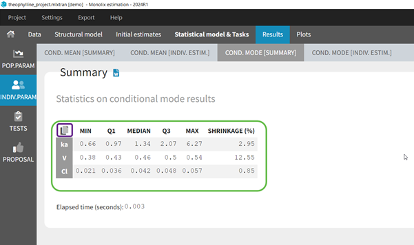
To see the estimated parameter value for each individual, the user can click on the [INDIV. ESTIM.] section. Notice that the user can also see them in the output files, which can be accessed via the folder icon at the bottom left. Notice that there is a “Copy table” icon on the top of each table to copy them in Excel, Word, … The table format and display will be kept.
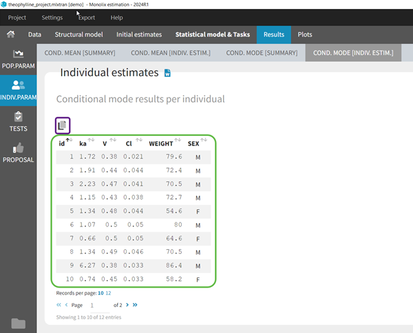
In the output folder
After having run the EBEs task, the following files are available:
- summary.txt: contains the summary statistics (as displayed in the GUI).
- IndividualParameters/estimatedIndividualParameters.txt: the individual parameters for each subject-occasion are displayed. In addition to the already present approximation conditional mean from SAEM (*_SAEM), the conditional mode (*_mode) is added to the file.
- IndividualParameters/estimatedRandomEffects.txt: the individual random effects for each subject-occasion are displayed (*_mode), in addition to the already present value based on the approximate conditional mean from SAEM (*_SAEM).
- IndividualParameters/shrinkage.txt: starting with Monolix 2024, the shrinkage for each parameter for the conditional mode as shrinkage_mode.
More details about the content of the output files can be found here.
Settings
The settings are accessible through the interface via the button next to the EBEs task.
![]()
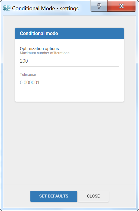
- Maximum number of iterations (default: 200): maximum number of iterations for the Nelder-Mead Simplex algorithm, for each individual. Even if the tolerance criteria is not met, the algorithm stops after that number of iterations.
- Tolerance (default: 1e-6): absolute tolerance criteria. The algorithm stops when the change of the conditional probability value between two iterations is less than the tolerance.
Calculate EBEs for a new data set using an existing model
5.1.4.Conditional distribution
- Purpose
- Calculation of the conditional distribution
- Conditional distribution
- MCMC algorithm
- Conditional mean
- Samples from the conditional distribution
- Stopping criteria
- Running the conditional distribution estimation task
- Outputs
- In the graphical user interface
- In the output folder
- Settings
Purpose
The conditional distribution represents the uncertainty of the individual parameter values. The conditional distribution estimation task permits to sample from this distribution. The samples are used to calculate the condition mean, or directly as estimators of the individual parameters in the plots to improve their informativeness [1]. They are also used to compute the statistical tests.
Calculation of the conditional distribution
Conditional distribution
The conditional distribution is \(p(\psi_i|y_i;\hat{\theta})\) with \(\psi_i\) the individual parameters for individual i, \(\hat{\theta}\) the estimated population parameters, and \(y_i\) the data (observations) for individual i. The conditional distribution represents the uncertainty of the individual’s parameter value, taking into account the information at hand for this individual:
- the observed data for that individual,
- the covariate values for that individual,
- and the fact that the individual belongs to the population for which we have already estimated the typical parameter value (fixed effects) and the variability (standard deviation of the random effects).
It is not possible to directly calculate the probability for a given \(\psi_i\) (no closed form), but is possible to obtain samples from the distribution using a Markov-Chain Monte-Carlo procedure (MCMC).
MCMC algorithm
MCMC methods are a class of algorithms for sampling from probability distributions for which direct sampling is difficult. They consist of constructing a stochastic procedure which, in its stationary state, yields draws from the probability distribution of interest. Among the MCMC class, we use the Metropolis-Hastings (MH) algorithm, which has the property of being able to sample probability distributions which can be computed up to a constant. This is the case for our conditional distribution, which can be rewritten as:
$$p(\psi_i|y_i)=\frac{p(y_i|\psi_i)p(\psi_i)}{p(y_i)}$$
\(p(y_i|\psi_i)\) is the conditional density function of the data when knowing the individual parameter values and can be computed (closed form solution). \(p(\psi_i)\) is the density function for the individual parameters and can also be computed. The likelihood \(p(y_i)\) has no closed form solution but it is constant.
In brief, the MH algorithm works in the following way: at each iteration k, a new individual parameter value is drawn from a proposal distribution for each individual. The new value is accepted with a probability that depends on \(p(\psi_i)\) and \(p(y_i|\psi_i)\). After a transition period, the algorithm reaches a stationary state where the accepted values follow the conditional distribution probability \(p(\psi_i|y_i)\). For the proposal distribution, three different distributions are used in turn with a (2,2,2) pattern (setting “Number of iterations of kernel 1/2/3” in Settings > Project Settings): the population distribution, a unidimensional Gaussian random walk, or a multidimensional Gaussian random walk. For the random walks, the variance of the Gaussian is automatically adapted to reach an optimal acceptance ratio (“target acceptance ratio” setting in Settings > Project Settings).
Conditional mean
The draws from the conditional distribution generated by the MCMC algorithm can be used to estimate any summary statistics of the distribution (mean, standard deviation, quantiles, etc). In particular we calculate the conditional mean by averaging over all draws:
$$ \hat{\psi}_i^{mean} = \frac{1}{K}\sum_{k=1}^{K}\psi_i^{k}$$
The standard deviation of the conditional distribution is also calculated. The number of samples used to calculate the mean and standard deviation corresponds to the number of chains times the total number of iterations of the conditional distribution task (not only during the convergence interval length). The mean is calculated over the transformed individual parameters (in the gaussian space), and back-transformed to the non-gaussian space.
Samples from the conditional distribution
Among all samples from the conditional distribution, a small number (between 1 and 10, see “Simulated parameters per individual” setting) is kept to be used in the plots. These samples are unbiased estimators and they present the advantage of not being affected by shrinkage, as shown for example on the documentation of the plot “distribution of the individual parameters“.
Stopping criteria
At iteration k, the conditional mean is calculated for each individual by averaging over all k previous iterations. The average conditional means over all individuals (noted E(X|y)), and the standard deviation of the conditional means over all individuals (noted sd(X|y)) are calculated and displayed in the pop-up window. The algorithm stops when, for all parameters, the average conditional means and standard deviations of the last 50 iterations (“Interval length” setting) do not deviate by more than 5% (2.5% in each direction, “relative interval” setting) from the average and standard deviation values at iteration k.
In some very specific cases (for example with a parameter with a normal distribution and a value very close to 1), it can take many iterations to reach the convergence criteria because the criteria is defined as a percentage. In that case, the toggle “enable maximum number of iterations” can be used to limit the number iterations of this task. If the limit is reached, a warning message will be displayed in the interface.
Running the conditional distribution estimation task
During the evaluation of the conditional distribution, the following plot pop-ups, displaying the average conditional means over all individuals (noted E(X|y)), and the standard deviation of the conditional means over all individuals (noted sd(X|y)) for each iteration of the MCMC algorithm.

The convergence criteria described above means that the blue line, which represents the average over all individuals of the conditional mean, must be within the tube. The tube is centered around the last value of the blue line and spans over 5% of that last value. The algorithm stops when all blue lines are in their tube.
Dependencies between tasks:
- The “Population parameters” task must be run before launching the conditional distribution task.
- The conditional distribution task is recommended before calculating the log-likelihood task without the linearization method (i.e log-likelihood via importance sampling).
- The conditional distribution task is necessary for the statistical tests.
- The samples generated during the conditional distribution task will be reused for the Standard errors task (without linearization).
Outputs
In the graphical user interface
In the Indiv.Param section of the Results tab, a summary of the estimated conditional mean is given (min, max, quartiles, and shrinkage [in Monolix 2024 and later]), as shown in the figure below. Starting from Monolix2021R1, the number of iterations is also displayed, along with a message indicating whether convergence has been reached (“auto-stop”) or if the task was stopped by the user or reached the maximum number of iterations.
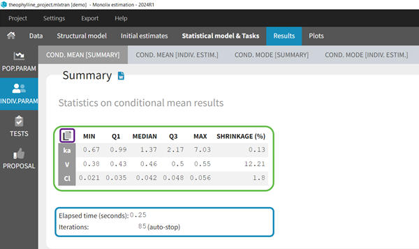
To see the estimated parameter value for each individual, the user can click on the [INDIV. ESTIM.] section. Notice that the user can also see them in the output files, which can be accessed via the folder icon at the bottom left. Notice that there is a “Copy table” icon on the top of each table to copy them in Excel, Word, … The table format and display will be kept.
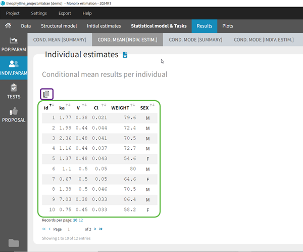
In the output folder
After having run the conditional distribution task, the following files are available:
- summary.txt: contains the summary statistics (as displayed in the GUI)
- IndividualParameters/estimatedIndividualParameters.txt: the individual parameters for each subject-occasion are displayed. The conditional mean (*_mean) and the standard deviation (*_sd) of the conditional distribution are added to the file. The number of samples used to calculate the mean and standard deviation corresponds to the number of chains times the total number of iterations of the conditional distribution task (not only during the convergence interval length).
- IndividualParameters/estimatedRandomEffects.txt: the individual random effects for each subject-occasion are displayed. Those corresponding to the conditional mean (*_mean) are added to the file, together with the standard deviation (*_sd).
- IndividualParameters/simulatedIndividualParameters.txt: several simulated individual parameters (draws from the conditional distribution) are recorded for each individual. The rep column permits to distinguish the several simulated parameters for each individual.
- IndividualParameters/simulatedRandomEffects.txt: the random effects corresponding to the simulated individual parameters are recorded.
- IndividualParameters/shrinkage.txt: starting with Monolix 2024, the shrinkage for each parameter for the conditional mean as shrinkage_mean and for the conditional distribution as shrinkage_condDist.
More details about the content of the output files can be found here.
Settings
To change the settings, you can click on the settings button next the conditional distribution task.

- Interval length (default: 50): number of iterations over which the convergence criteria is checked.
- Relative interval (default: 0.05): size of the interval (relative to the current average or standard deviation) in which the last “interval length” iterations must be for the stopping criteria to be met. A value at 0.05 means that over the last “interval length” iterations, the value should not vary by more than 5% (2.5% in each direction).
- Simulated parameters per individual (default: via calculation): number of draws from the conditional distribution that will be used in the plots. The number is calculated as min(10, idealNb) with idealNb = max(500 / number of subject , 5000 / number of observations). This means that the maximum number is 10 (which is usually the case for small data sets). For large data sets, the number may be reduced, but the number of individual times the number of simulated parameters should be at least 500, and the number of observations times the number of simulated parameters should be at least 5000. This ensures to have a sufficiently large but not unnecessarily large number of dots in the plots such as Observations versus predictions or Correlation between random effects.
If the user sets the number of simulated parameters to a value larger than the number of chains (project settings) times the total number of iterations of the conditional distribution task (maximum number of iterations or when convergence criteria are reached), the number will be restricted to the number of available samples.
If the user sets the number of simulated parameters to a value smaller than interval length times number of chains, the simulated parameters are picked evenly from the interval length and the chains. If the requested number of simulated parameters is larger, the last n (n=number of requested simulated parameters) samples are picked. - Enable maximum iterations limit (default: toggle off) [from version 2020 on]: When the toggle in “on”, a maximum number of iterations can be defined.
- Maximum number of iterations (default: 500, needs to be larger than the interval length, available if “enable maximum iterations limit’ is on): maximum number of iterations for the conditional distribution task. Even if the convergence criteria are not fulfilled, the algorithm stops after this maximum number of iterations. If the maximum number of iterations is reached, a warning message will be displayed in the interface.
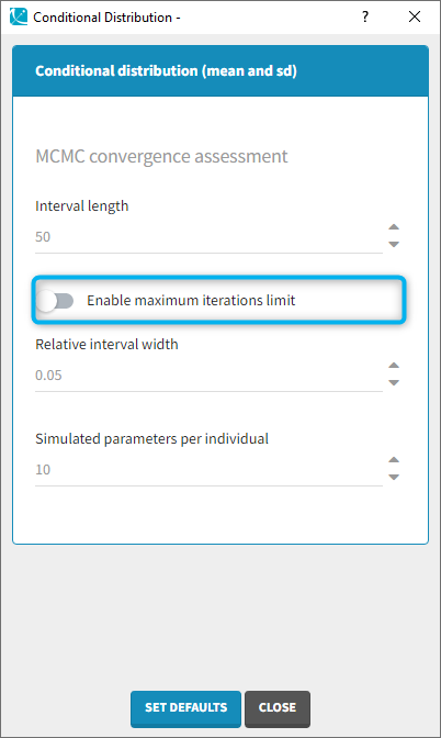 |
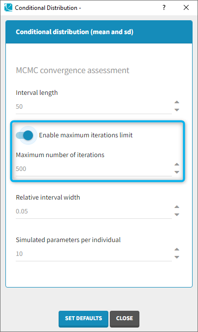 |
|---|
5.1.4.1.Understanding shrinkage and how to circumvent it
- Introduction
- Conditional distribution
- Conditional mode (EBEs) and conditional mean
- Shrinkage
- Consequences of shrinkage
- How to circumvent shrinkage
- Example
- Conclusion
Introduction
Shrinkage is a phenomenon that appears when the data is insufficient to precisely estimate the individual parameters (EBEs). In that case, the EBEs “shrink” towards the center of the population distribution and do not properly represent the inter-individual variability. This leads to diagnostic plots that may be misleading, either hiding true relationships or inducing wrong ones.
In the diagnostic plots, Monolix uses samples from the conditional distribution as individual parameters, which lead to reliable plots even when shrinkage is present in the model [1]. This method is based on the calculation of the conditional distribution.
Conditional distribution
The conditional distribution is defined for each individual. It represents the uncertainty of the individual’s parameter value, taking the information at hand for this individual into account:
- the observed data for that individual,
- the covariate values for that individual,
- the fact that the individual belongs to the population for which we have already estimated the typical parameter value (fixed effects) and the inter-individual variability (standard deviation of the random effects).
In a mathematical formalism, the conditional distribution is written \(p(\psi_i|y_i;\hat{\theta})\) with \(\psi_i\) the individual parameters for individual \(i\), \(\hat{\theta}\) the estimated population parameters, and \(y_i\) the data (observations) for individual \(i\).
It is not possible to directly calculate the probability for a given \(\psi_i\) (no closed form), but it is possible to obtain samples from the distribution using a Markov-Chain Monte-Carlo procedure (MCMC). This is what is done in the Conditional distribution task.
With the following conditional distribution for the volume V of individual i, we see that the most probable value is around 25 L but there is quite some uncertainty: the value could also be 15 or 40 for instance. For visual purpose, we have drawn the distribution as a smooth curve, but remember that the conditional distribution has no explicit expression. One can only obtain samples from this distribution using MCMC.
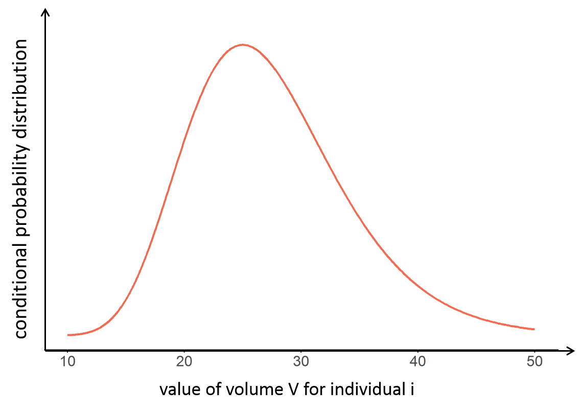
Conditional mode (EBEs) and conditional mean
It is often convenient to work with a single value for the individual parameters (called an estimator), instead of a probability distribution. Several “summary” values can be used, such as the mode or the mean of the conditional distribution.
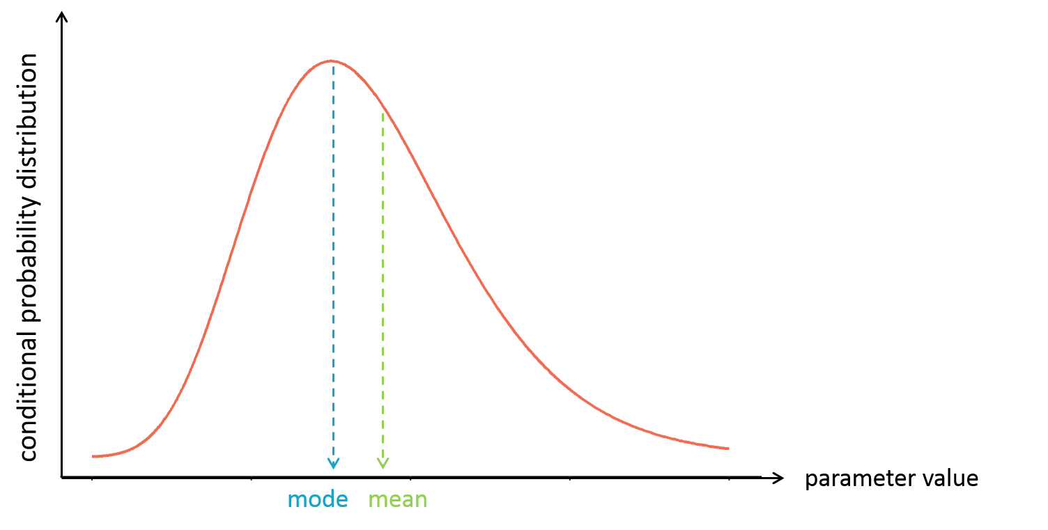
The mode is also called maximum a posteriori or EBE (for empirical bayes estimate). It is often preferred over the mean, because the mode represents the most likely value, i.e the value which has the highest probability.
In Monolix, the mode is calculated via the EBEs task, while the mean is calculated via the Conditional distribution task, as the average of all samples drawn from the conditional distribution.
Once the value of the individual estimator (conditional mode or conditional mean) is known for each individual, one can easily calculate the individual random effects for each individual. For instance for the volume V, that depends on the covariate weight WT:
$$\begin{array}{rl} V_i& = V_{pop}\left(\frac{\textrm{WT}_i}{70}\right)^{\beta}e^{\eta_i} \\ \Rightarrow \quad \eta_i& = \log (V_i) – \log(V_{pop}) – \beta \log \left(\frac{\textrm{WT}_i}{70}\right) \end{array} $$
The individual parameters and individual random effects are used in diagnostic plots. They are used either directly, such as in the Correlation between random effects or Individual parameter versus covariate plots, or indirectly to generate individual predictions, such as in Individual Fits, Observations versus Predictions or Scatter plot of the residuals. But these diagnostic plots can be biased in presence of shrinkage.
Shrinkage
When the individual data brings only few information about the individual parameter value, the conditional distribution is large, reflecting the uncertainty of the individual parameter value. In that case, the mode of the conditional distribution is close to (or “shrinks” to) the mode of the population distribution. If this is the case for all or most of the individuals, all individual parameters end up concentrated around the mode of the population distribution and do not correctly represent the inter-individual variability which has been estimated via the standard deviation parameters (omega parameters in Monolix). This is the shrinkage phenomenon. Shrinkage typically occurs when the data is sparse.
Below we present the example of a parameter V which has a lot of shrinkage and a parameter k with almost no shrinkage. We consider a data set with 10 individuals. In the upper plots, the conditional distributions of each of the 10 individuals are shown. For the volume V, the individual parameter values are uncertain and their conditional distributions are large. When reporting the mode (closed circles) of the conditional distributions on the population distribution (black curve, bottom plots), the modes appear shrunk compared to the population distribution. On the opposite, for k, the conditional distributions are narrow and the modes are well spread over the population distribution. There is shrinkage for V, but not for k.
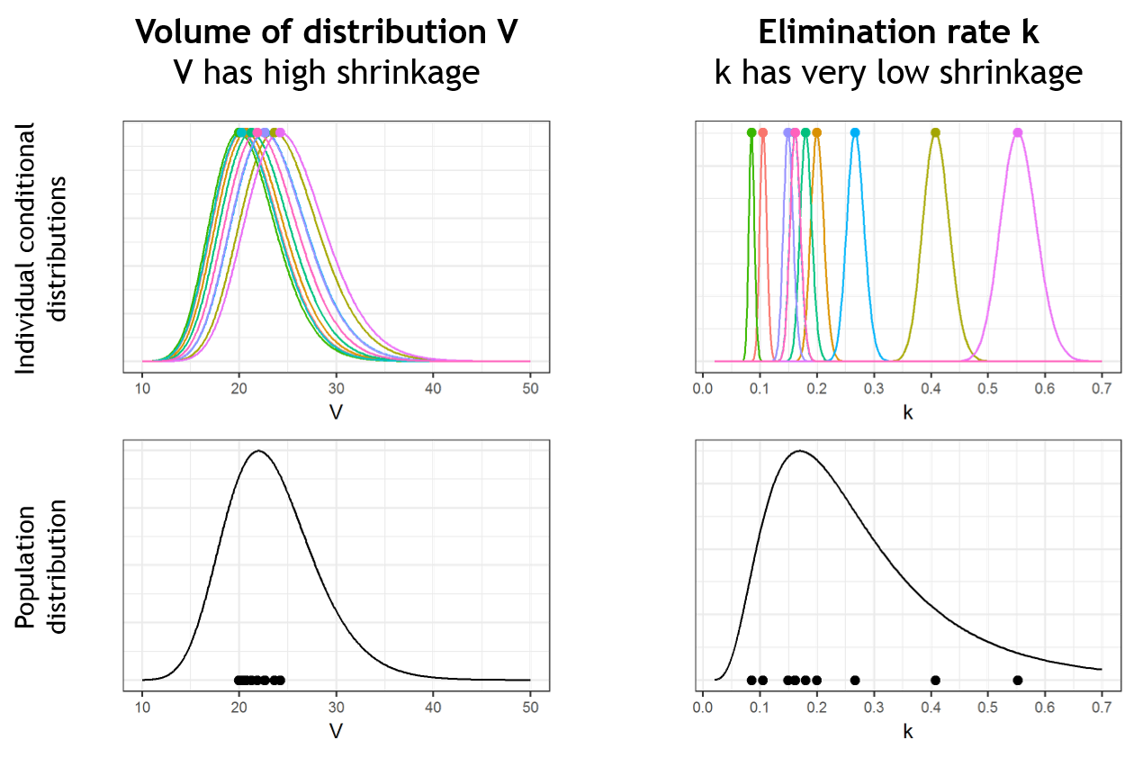
Pulling the individual parameters of all individuals together, one can overlay the population distribution (black line) with the histogram of individual parameters (i.e conditional modes) (blue bars). This is displayed in the Distribution of the individual parameters plot in Monolix:
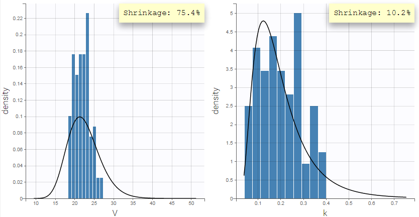
The shrinkage phenomenon can be quantified via a shrinkage value for each parameter. In Monolix, the formula for shrinkage has been updated in version 2024 to use the standard deviation instead of the variance in accordance with industry standards.
Starting with Monolix version 2024, shrinkage is calculated from the empirical standard deviation of the random effects \( \textrm{sd}(\eta_i) \) and the estimated standard deviation (the omega population parameter \(\omega\)). The random effects \( \textrm{sd}(\eta_i) \) can be calculated from the EBEs, conditional mean or samples from the conditional distribution. Typically, the shrinkage is reported using the EBEs.
$$\eta\textrm{-sh}=1-\frac{\textrm{sd}(\eta_i)}{\omega}$$
In the case of inter occasion variability, shrinkage includes both inter individual and inter occasion variability (the gamma population parameter \(\gamma\))
$$\eta\textrm{-sh}=1-\frac{\textrm{sd}(\eta_i)}{\sqrt{\omega^2 + \gamma^2}}$$
In Monolix versions 2023 and earlier, shrinkage is calculated using the ratio of the empirical variance and the estimated variance as:
$$\eta\textrm{-sh}=1-\frac{\textrm{var}(\eta_i)}{\omega^2}$$
Results
In Monolix versions 2023 and earlier, the shrinkage can be displayed in the Distribution of the individual parameters plot, by selecting the “information” toggle.
Starting in Monolix version 2024, shrinkage information is available in several ways:
- Results / Indiv. Results / Cond. Mean [summary] – shrinkage is reported if the Conditional Distribution task has been run
- Results / Indiv. Results / Cond. Mode [summary] – shrinkage is reported if the EBEs task has been run
- In the IndividualParameters folder inside the results folder, there is a file shrinkage.txt
- In reports, using the metric SHRINKAGE in the population or individual parameters table placeholder
- In the plot Distribution of the individual parameters by switching on “information”
- In the plot Distribution of the standardized random effects by switching on “information”
Calculating the shrinkage in R
Starting with Monolix version 2024, there is a method available to directly return the shrinkage information: getEtaShrinkage().
In Monolix version 2023 and earlier, there is no function from the lixoftConnectors to directly get the shrinkage, but you can easily calculate it from the estimated parameters like this for example for parameter V:
population_params <- read.csv("monolix_project/populationParameters.txt")
eta_estimated <- read.csv("monolix_project/IndividualParameters/estimatedRandomEffects.txt")
omega_V <- population_params$value[population_params$parameter=="V"]
eta_V_estimated_mode <- eta_estimated$eta_V_mode
shrinkage_eta_V_estimated_mode <- (1-var(eta_V_estimated_mode)/omega_V^2)*100
Comparison to Nonmem: the Nonmem definition of shrinkage is based on a ratio of standard deviations. This is also the case in Monolix 2024 and above. However, Monolix 2023 and below uses a ratio of variances (which is more common in statistics). Below we provide a “conversion table” which should be read in the following way: a situation that would in Nonmem and Monolix 2024 lead to a shrinkage calculation of 30%, would in Monolix 2023 lead to a calculation of shrinkage of around 50%. The Nonmem and Monolix 2024 version of the shrinkage can be calculated from the Monolix 2023 shrinkage using the following formula:
$$\eta\textrm{-shNM}=\eta\textrm{-shMLX24}=1-\sqrt{1-\eta\textrm{-shMLX23}}$$
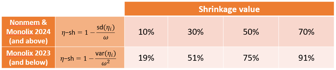
Is it OK to get a negative shrinkage? Yes. In case of no shrinkage, \(var(\eta_i)= \omega^2\) when \(var(\eta_i)\) is calculated on an infinitely large sample. In practice, \(var(\eta_i)\) is calculated on a limited sample related to the number of individuals. Its value can be by chance a little bigger than \(\omega^2\), leading to a slightly negative shrinkage.
Consequences of shrinkage
In case of shrinkage the individual parameters (conditional mode/EBEs or conditional mean) are biased because they do not correctly reflect the population distribution.
As these individual parameters are used in diagnostic plots (in particular the Correlation between random effects and the Individual parameters versus covariates plots) the diagnostic plots can become misleading in presence of shrinkage, either hiding relations or suggesting wrong ones. This complicates the identification of mis-specifications and burdens the modeling process.
Note that the shrinkage of the EBEs has no consequences on the population parameter estimation via SAEM (which doesn’t use EBEs, contrary to FOCE for instance). However the lack of informative data may lead to large standard errors for the population parameters and a slower convergence.
How to circumvent shrinkage
Monolix provides a very efficient solution to circumvent the shrinkage problem, i.e the bias in the diagnostic plots induced by the use of shrunk individual parameters. Instead of using the shrunk conditional mode/EBEs or conditional mean, Monolix uses parameter values randomly sampled from the conditional distribution:

The fact of pooling the random samples of the conditional distribution of all individuals allows us to look at them as if they where sampled from the population distribution. And this is exactly what we want: to have individual parameter values (i.e the samples) that correctly reflect the population distribution.
From a mathematical point of view, one can show that the random samples are an unbiased estimator:
$$p(\psi_i)=\int p(\psi_i|y_i)p(y_i)dy_i=\mathbb{E}_{y_i}(p(\psi_i|y_i))$$
The improvement brought by the random samples from the conditional distributions can be visualized in the following way: while the mode (closed circles) are shrunk, the random samples (stars) spread over the entire population distribution (in black). One can even draw several random sample per individual to increase the informativeness of the diagnostic plots. This is what is done in the MonolixSuite2018R1 version (while MonolixSuite2016R1 uses one sample per individual).
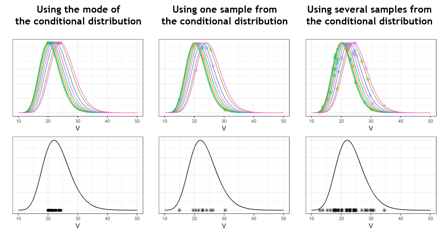
In [1], the authors warrant the use of sampled individual parameters. They demonstrate their usefulness in diagnostic plots via numerical experiments with simulated data. They also show that statistical tests based on these sampled individual parameters are unbiased, the type I error rate is the desired significance level of the test and the probability to detect a mis-specification in the model increases with the magnitude of this mis-specification.
Example
Fitting the sparse Tobramycin data with a (V,k) model leads to a high shrinkage (75%) of the volume V when using the EBEs. On the opposite, when using samples from the conditional distributions of each individual, there is no shrinkage anymore.
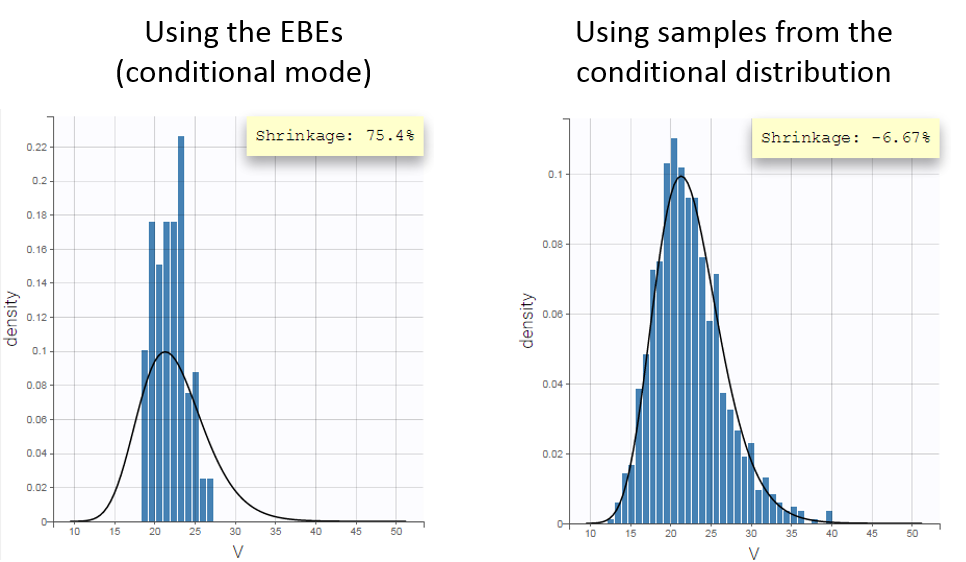
The usefulness of using the samples from the conditional distribution can be seen in the Correlation between the random effects plot. Using the EBEs, the plot suggests a positive correlation of about 30% between the volume and the elimination rate. Using the random samples, the plot does not suggest this correlation any more. If the correlation is added to the model, it is estimated small and not significant.
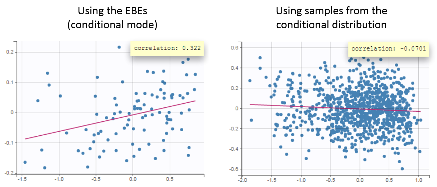
Another example of shrinkage can be seen for the parameter ka in the warfarin data set. In this example, the data is sparse during the absorption phase leading to a large uncertainty of the individual parameter values.
Conclusion
The use of samples from the conditional distribution is a powerful way to avoid the bias due to the shrinkage in the diagnostic plots. This method has been validated mathematically and with numerical experiments.
In Monolix, the random samples are used by default in all diagnostic plots, if the Conditional distribution task has been run. The choice of the estimator for the individual parameters can be changed in the Settings tab:
5.1.4.2.Statistical tests
Several statistical tests may be automatically performed to test the different components of the model. These tests use individual parameters drawn from the conditional distribution, which means that you need to run the task “Conditional distribution” in order to get these results. In addition, the tests for the residuals require to have first generated the residuals diagnostic plots (scatter plot or distribution).
The tests are all performed using the individual parameters sampled from the conditional distribution (or the random effects and residuals derived thereof). They are thus not subject to bias in case of shrinkage. For each individual, several samples from the conditional distribution may be used. The used tests include a correction to take into account that these samples are correlated among each other.
Results of the tests are available in the tab “Results” and selecting “Tests” in the left menu
The model for the individual parameters
Consider a PK example (warfarin data set from the demos) with the following model for the individual PK parameters (ka, V, Cl):
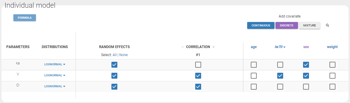
In this example, the different assumptions we make about the model are:
- The 3 parameters are lognormally distributed
- ka is function of sex
- V is function of sex and weight. More precisely, the log-volume log(V) is a linear function of the log-weight \({\rm lw70 }= \log({\rm wt}/70)\).
- Cl is not function of any of the covariates.
- The random effects \(\eta_V\) and \(\eta_{Cl}\) are linearly correlated
- \(\eta_{ka}\) is not correlated with \(\eta_V\) and \(\eta_{Cl}\)
Let’s see how each of these assumptions are tested:
Covariate model
Individual parameters vs covariates – Test whether covariates should be removed from the model
If an individual parameter is function of a continuous covariate, the linear correlation between the transformed parameter and the covariate is not 0 and the associated \(\beta\) coefficient is not 0 either. To detect covariates bringing redundant information, we check if these beta coefficients are different from 0. For this, we perform two different tests: a correlation test based on betas coefficients estimated with a linear regression, and a Wald test relying on the estimated population parameters and their standard error.
In both cases, a small p-value indicates that the null hypothesis can be rejected and thus that the estimated beta parameter is significantly different from zero. If this is the case, the covariate should be kept in the model. On the opposite, if the p-value is large, the null hypothesis cannot be rejected and this suggests to remove the covariate from the model. Note that if beta is equal to zero, then the covariate has no impact on the parameter. High p-values are colored in yellow (p-value in [0.01-0.05]), orange (p-value in [0.05-0.10]) or red (p-value in [0.10-1]) to draw attention on parameter-covariate relationships that can be removed from the model from a statistical point of view.
Correlation test
Briefly, we perform a linear regression between the covariates and the transformed parameters and test if the resulting beta coefficient are different from 0.
More precisely: for each individual \(i\), let \(z_i^l\) be the transformed individual parameters (e.g log(V) for log-normally distributed parameters or logit(F) for logit-distributed parameters) sampled from the conditional distribution (called replicates, index l). Here we will call covariates all continuous covariates and all non-referent categories of categorical covariates \(cov^{(c)}, c = 1..n_C\). For each individual \(i\), \(cov_i^{(c)}\) is the value of the c\(^{th}\) covariate, equal to 0 or 1 if the covariate is a category.
The transformed individual parameters are first averaged over replicates for each individual:
$$z_i^{(L)}=\frac{1}{L} \sum_{l=1}^{L} z_i^l$$
We then perform the following linear regression:
$$z_i^{(L)}=\alpha_0 + \sum_{c=1}^{n_c} \beta_c \text{cov}_i^{(c)} + e_i$$
If two covariates \(cov^{(1)}\) and \(cov^{(2)}\) (for example WT and BMI) are strongly correlated with a parameter \(z^{(L)}\) (for example the volume), only one of them is needed in the model because they are redundant. In the linear regression, only one of the estimated \(\hat{\beta_1}\) and \(\hat{\beta_2}\) will be significantly different from zero.
For each covariate \(c\) we conduct a t-test on the \(\hat{\beta_c}\) with the null hypothesis:
H0: \(\beta_c = 0\).
The test statistic is
$$T_0 = \frac{\hat{\beta_c}}{se(\hat{\beta_c})}$$
where \(se(\hat{\beta_c})\) is the estimated standard error of \(\hat{\beta_c}\) (obtained by least squares estimation during the regression). If the null hypothesis is true, \(T_0\) follows a t distribution with \(N-n_C-1\) degrees of freedom (where N is the number of individuals).
In our example, the correlation test suggests to remove sex from ka:
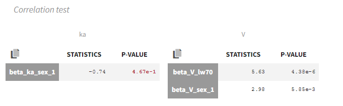
Wald test
The Wald test relies on the standard errors. Thus the task “Standard errors” must have been calculated to see the test results. The test can be performed using the standard errors calculated using either the “linearization method” (indicated as “linearization”) or not (indicated as “stochastic approximation” in the tests).
The Wald test tests the following null hypothesis:
H0: the beta parameter estimated by SAEM is equal to zero.
The math behind: Let’s note \( \hat{\beta} \) the estimated beta value (which is a population parameter) and \(se(\hat{\beta}) \) the associated standard error calculated during the task “Standard errors”. The Wald test statistic is:
$$W=\frac{\hat{\beta}}{se(\hat{\beta})} $$
The test statistic is compared to a normal distribution (z distribution).
In our example, the Wald test suggests to remove sex from ka and V:
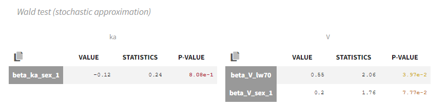
Remark: the Wald test and the correlation test may suggest different covariates to keep or remove. Note that the null hypothesis tested is not the same.
Random effects vs covariates – Test whether covariates should be added to the model
Pearson’s correlation tests and ANOVA are performed to check if some relationships between random effects and covariates not yet included in the model should be added to the model.
For continuous covariates, the Pearson’s correlation test tests the following null hypothesis:
H0: the person correlation coefficient between the random effects (calculated from the individual parameters sampled from the conditional distribution) and the covariate values is zero
For categorical covariates, the one-way ANOVA tests the following null-hypothesis:
H0: the mean of the random effects (calculated from the individual parameters sampled from the conditional distribution) is the same for each category of the categorical covariate
A small p-value indicates that the null hypothesis can be rejected and thus that the correlation between the random effects and the covariate values is significant. If this is the case, it is probably worth considering to add the covariate in the model. Note that the decision of adding a covariate in the model should not only be driven by statistical considerations but also biological relevance. Note also that for parameter-covariate relationships already included in the model, the correlation between the random effects and covariates is not significant (while the correlation between the parameter and the covariate can be – see above). Small p-values are colored in yellow (p-value in [0.05-0.10]), orange (p-value in [0.01-0.05]) or red (p-value in [0.00-0.01]) to draw attention on parameter-covariate relationships that can be considered for addition in the model from a statistical point of view.
In our example, we already have sex on ka and V, and lw70 on V in the model. The only remaining relationship that could possibly be worth investigating is between weight (or the log-transformed weight “lw70”) and clearance.
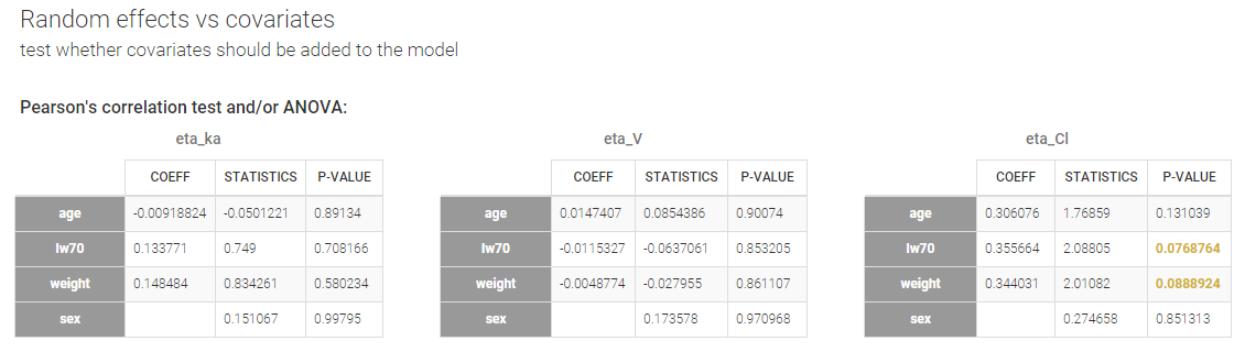
The math behind:
Continuous covariate: Let \(\eta_i^l\) the random effects corresponding to the \(L\) individual parameters sampled from the conditional distribution (called replicates) for individual \(i\), and \(cov_i\) the covariate value for individual \(i\). The random effects are first averaged over replicates for each individual:
$$ \eta_i^{(L)}=\frac{1}{L} \sum_{l=1}^{L} \eta_i^l $$
We note \(\overline{cov} = \sum_{i=1}^N cov_i \) the average covariate value over the N subjects and \(\overline{\eta}=\sum_{i=1}^N \eta_i^{(L)} \) the average random effect. The Pearson correlation coefficient is calculated as:
$$r=\frac{\sum_{i=1}^N(cov_i – \overline{cov})(\eta_i^{(L)} – \overline{\eta})}{\sqrt{ \sum_{i=1}^N(cov_i – \overline{cov})^2 \sum_{i=1}^N(\eta_i^{(L)} – \overline{\eta})^2}}$$
The test statistic is:
$$t=\frac{r}{\sqrt{1-r^2}}\sqrt{N-2}$$
and it is compared to a t-distribution with \(N-2\) degrees of freedom with \(N\) the number of individuals.
Categorical covariates: The random effects are first averaged over replicates for each individual and a one-way analysis of variance is performed (simplified to a t-test when the covariate has only two categories).
The model for the random effects
Distribution of the random effects – Test if the random effects are normally distributed
In the individual model, the distributions for the parameters assume that the random effects follow a normal distribution. Shapiro-Wilk tests are performed to test this hypothesis. The null hypothesis is:
H0: the random effects are normally distributed
If the p-value is small, there is evidence that the random effects are not normally distributed and this calls the choice of the individual model (parameter distribution and covariates) into question. Small p-values are colored in yellow (p-value in [0.05-0.10]), orange (p-value in [0.01-0.05]) or red (p-value in [0.00-0.01]).
In our example, there is no reason to reject the null-hypothesis and no reason to question the chosen log-normal distributions for the parameters.
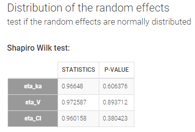
The math behind: Let \(\eta_i^l\) the random effects corresponding to the \(L\) individual parameters sampled from the conditional distribution (called replicates) for individual \(i\). The Shapiro-Wilk test statistic is calculated for each replicate \(l\) (i.e the first sample from all individuals, then the second sample from all individuals, etc):
$$W^l=\frac{\left( \sum_{i=1}^N a_i \eta_i^l \right)^2}{ \sum_{i=1}^N (\eta_i^l – \overline{\eta}^l)^2}$$
with \(a_i\) tabulated coefficient and \(\overline{\eta}^l=\frac{1}{N}\sum_{i=1}^N \eta_i^l \) the average over all individuals, for each replicate.
The statistic displayed in Monolix corresponds to the average statistic over all replicates \(W=\frac{1}{L}\sum_{l=1}^L W^l \). For the p-values, one p-value is calculated for each replicate, using the Shapiro-Wild table with \(N\) (number of individuals) degrees of freedom. The Benjamini-Hochberg (BH) procedure is then applied: the p-values are ranked by ascending order and the BH critical value is calculated for each as \( \frac{\textrm{rank}}{L}Q \) with \(\textrm{rank}\) the individual p-value’s rank, \(L\) the total number of p-values (equal to the number of replicates) and \(Q=0.05\) the false discovery rate. The largest p-value that is smaller than the corresponding critical value is selected.
Joint distribution of the random effects – Test if the random effects are correlated
Correlation tests are performed to test if the random effects (calculated from the individual parameters sampled from the conditional distribution) are correlated. The null-hypothesis is:
H0: the expectation of the product of the random effects of the first and second parameter is zero
The null-hypothesis is assessed using a t-test.
Remark: In the 2018 version, a Pearson correlation test was used.
For correlations not yet included in the model, a small p-value indicates that there is a significant correlation between the random effects of two parameters and that this correlation should be estimated as part of the model (otherwise simulations from the model will assume that the random effects of the two parameters are not correlated, which is not what is observed for the random effects estimated using the data). Small p-values are colored in yellow (p-value in [0.05-0.10]), orange (p-value in [0.01-0.05]) or red (p-value in [0.00-0.01]).
For correlations already included in the model, a large p-value indicates that one cannot reject the hypothesis that the correlation between the random effects is zero. If the correlation is not significantly different from zero, it may not be worth estimating it in the model. High p-values are colored in yellow (p-value in [0.01-0.05]), orange (p-value in [0.05-0.10]) or red (p-value in [0.10-1])
In our example, we have assumed in the model that \(\eta_V\) and \(\eta_{Cl}\) are correlated. The high p-value (0.033, above the 0.01 threshold, see above) indicates that the correlation between the random effects of V and Cl is not significantly different from zero and suggests to remove this correlation from the model.
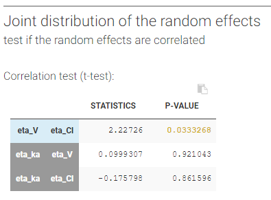
Remark: as correlations can only be estimated by groups (i.e if a correlation is estimated between (ka, V) and between (V, Cl), then one must also estimate the correlation between (ka, Cl)), it may happen that it is not possible to remove a non-significant correlation without removing also a significant one.
The math behind: Let \(\eta_{\psi_1,i}^l\) and \(\eta_{\psi_2,i}^l\) the random effects corresponding to the \(L\) individual parameters \(\psi_1\) and \(\psi_2\) sampled from the conditional distribution (called replicates) for individual \(i\). First we calculate the product of the random effects averaged over the replicates:
$$p_i^{(L)} = \frac{1}{L} \sum_{l=1}^{L} \eta_{\psi_1,i}^l \eta_{\psi_2,i}^l $$
We note \( \overline{p}=\sum_{i=1}^{N} p_i^{(L)} \) the average of the product over the individuals and \(s\) their standard deviation. The test statistic is:
$$ T=\frac{\overline{p}}{\frac{s}{\sqrt{N}}}$$
and it is compared to a t-distribution with \(N-1\) degrees of freedom with \(N\) the number of individuals.
The distribution of the individual parameters
Distribution of the individual parameters not dependent on covariates – Test if transformed individual parameters are normally distributed
When an individual parameter doesn’t depend on covariates, its distribution (normal, lognormal, logit or probit) can be transformed into the normal distribution. Then, a Shapiro-Wilk test can be used to test the normality of the transformed parameter. The null hypothesis is:
H0: the transformed individual parameter values (sampled from the conditional distribution) is normally distributed
If the p-value is small, there is evidence that the transformed individual parameter values are not normally distributed and this calls the choice of the parameter distribution into question. Small p-values are colored in yellow (p-value in [0.05-0.10]), orange (p-value in [0.01-0.05]) or red (p-value in [0.00-0.01]).
In our example, there is no reason to reject the null hypothesis of lognormality for Cl.
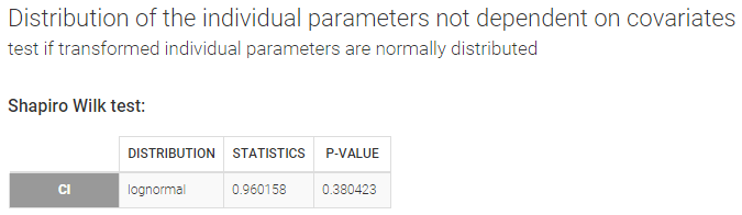
Remark: testing the normality of a transformed individual parameter that does not depend on covariates is equivalent to testing the normality of the associated random effect. We can check in our example that the Shapiro-Wilk tests for \(\log(Cl)\) and \(\eta_{Cl}\) are equivalent.
The math behind: Let \(z_i^l\) the transformed individual parameters (e.g log(V) for log-normally distributed parameters and logit(F) for logit-distributed parameters) sampled from the conditional distribution (called replicates, index \(l\) ) for individual \(i\). The Shapiro-Wilk test statistic is calculated for each replicate \(l\) (i.e the first sample from all individuals, then the second sample from all individuals, etc):
$$W^l=\frac{\left( \sum_{i=1}^N a_i z_i^l \right)^2}{ \sum_{i=1}^N (z_i^l – \overline{z}^l)^2}$$
with \(a_i\) tabulated coefficient and \(\overline{z}^l=\frac{1}{N}\sum_{i=1}^N z_i^l \) the average over all individuals, for each replicate.
The statistic displayed in Monolix corresponds to the average statistic over all replicates \(W=\frac{1}{L}\sum_{l=1}^L W^l \). For the p-values, one p-value is calculated for each replicate, using the Shapiro-Wild table with \(N\) (number of individuals) degrees of freedom. The Benjamini-Hochberg (BH) procedure is then applied: the p-values are ranked by ascending order and the BH critical value is calculated for each as \( \frac{\textrm{rank}}{L}Q \) with \(\textrm{rank}\) the individual p-value’s rank, \(L\) the total number of p-values (equal to the number of replicates) and \(Q=0.05\) the false discovery rate. The largest p-value that is smaller than the corresponding critical value is selected.
Distribution of the individual parameters dependent on covariates – test the marginal distribution of each individual parameter
Individual parameters that depend on covariates are not anymore identically distributed. Each transformed individual parameter is normally distributed, with its own mean that depends on the value of the individual covariate. In other words, the distribution of an individual parameter is a mixture of (transformed) normal distributions. A Kolmogorov-Smirnov test is used for testing the distributional adequacy of these individual parameters. The null-hypothesis is:
H0: the individual parameters are samples from the mixture of transformed normal distributions (defined by the population parameters and the covariate values)
A small p-value indicates that the null hypothesis can be rejected. Small p-values are colored in yellow (p-value in [0.05-0.10]), orange (p-value in [0.01-0.05]) or red (p-value in [0.00-0.01]).
With our example, we obtain:
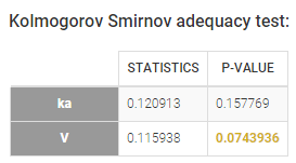
The model for the observations
A combined1 error model with a normal distribution is assumed in our example:
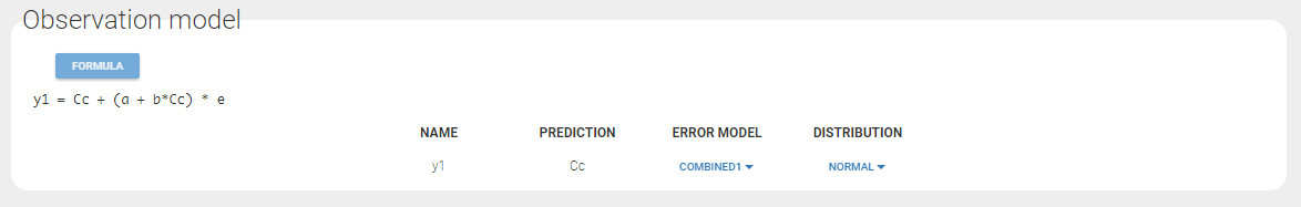
Distribution of the residuals
Several tests are performed for the individual residuals (IWRES), the NPDE and for the population residuals (PWRES).
Test if the distribution of the residuals is symmetrical around 0
A Miao, Gel and Gastwirth (2006) test (or Van Der Waerden test in the 2018 release) is used to test the symmetry of the residuals. Indeed, symmetry of the residuals around 0 is an important property that deserves to be tested, in order to decide, for instance, if some transformation of the observations should be done. The null hypothesis tested is:
H0: the median of the residuals is equal to its mean
A small p-value indicates that the null hypothesis can be rejected. Small p-values are colored in yellow (p-value in [0.05-0.10]), orange (p-value in [0.01-0.05]) or red (p-value in [0.00-0.01]).
With our example, we obtain:
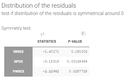
The math behind: Let \(R_i\) the residuals (NPDE, PWRES or IWRES) for each individual \(i\), \(\overline{R}\) the mean of the residuals, and \(M_R\) their median. The MGG test statistic is:
$$T=\frac{\sqrt{n}}{0.9468922}\frac{\overline{R}-M_R}{ \sum_{i=1}^{n}|R_i-M|}$$
with \(n\) the number of residuals. The test statistic is compared to a standard normal distribution.
The formula above is valid for i.i.d (independent and identically distributed) residuals. For the IWRES, the residuals corresponding to a given time and given id are not independent (they ressemble each other). To solve the problem, we estimate an effective number of residuals. The number of residuals \(n\) can be split into the number of replicates \(L\) times the number of observations \(m\). We look for the effective number of replicates \(\tilde{L}\) such that:
$$ \frac{\tilde{L}}{L} \sum_{l=1}^L (R_i^l)^2 \approx \chi^2(\tilde{L})$$
using a maximum likelihood estimation. The number of residuals is then calculated as \(n=\tilde{L} \times m \).
Test if the residuals are normally distributed
A Shapiro Wilk test is used for testing the normality of the residuals. The null hypothesis is:
H0: the residuals are normally distributed
If the p-value is small, there is evidence that the residuals are not normally distributed. The Shapiro Wilk test is known to be very powerful. Then, a small deviation of the empirical distribution from the normal distribution may lead to a very significant test (i.e. a very small p-value), which does not necessarily means that the model should be rejected. Thus, no color highlight is made for this test.
In our example, we obtain:
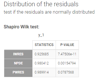
The math behind: Let \(R_i^l\) the residuals (NPDE, PWRES or IWRES) for individual \(i\). NPDE and PWRES have one values per time points and per individual. IWRES have one value per time point, per individual and per replicate (corresponding to the \(L\) individual parameters sampled from the conditional distribution). The Shapiro-Wilk test statistic is calculated for each replicate \(l\) (i.e the first sample from all individuals, then the second sample from all individuals, etc):
$$W^l=\frac{\left( \sum_{i=1}^N a_i R_i^l \right)^2}{ \sum_{i=1}^N (R_i^l – \overline{R}^l)^2}$$
with \(a_i\) tabulated coefficient and \(\overline{R}^l=\frac{1}{N}\sum_{i=1}^N R_i^l \) the average over all individuals, for each replicate.
The statistic displayed in Monolix corresponds to the average statistic over all replicates \(W=\frac{1}{L}\sum_{l=1}^L W^l \). For the p-values, one p-value is calculated for each replicate, using the Shapiro-Wild table with \(N\) (number of individuals) degrees of freedom. The Benjamini-Hochberg (BH) procedure is then applied: the p-values are ranked by ascending order and the BH critical value is calculated for each as \( \frac{\textrm{rank}}{L}Q \) with \(\textrm{rank}\) the individual p-value’s rank, \(L\) the total number of p-values (equal to the number of replicates) and \(Q=0.05\) the false discovery rate. The largest p-value that is smaller than the corresponding critical value is selected.
5.1.4.3.Proposal
Starting from the 2019 version, the section Proposal in the tab Results includes automatic proposals of improvements for the statistical model, based on comparisons of many correlation, covariate and error models.
Model selections are performed by using a BIC criteria (called Criteria in the interface), based on the current simulated individual parameters. This is why the proposal is computed by the task Conditional distribution.
Note that the BIC criteria is not the same as the BIC computed for the Monolix project with the task log-likelihood: it does not characterize the whole model but only each part of the statistical model evaluated in the proposal, and thus yields different values for each type of model. Each criteria is given by the formula:
\(BIC = -2\log({\cal L’})/nRep+\log(N) * k\),
where:
- \(\cal L’\) = likelihood of the linear regression
- N = number of individuals
- k = number of estimates betas
- nRep = number of replicates (samples per individual)
The number of estimated parameters k characterizes the part of the statistical model that is evaluated. The likelihood \(\cal L’\) is not the same as the one computed by the log-likelihood task, it is based on the joint distribution:
\(p(y_i, \phi_i; \theta)=p(y_i| \phi_i; \theta)p(\phi_i; \theta)\)
where all the parameters are fixed to the values estimated by Monolix except the parameters characterizing the model that is evaluated: error parameters (in \(\theta\)) for the error models, individual parameters or random effects (in \(\phi_i\)) for the covariate models or the correlation models.
Proposed model
The section Proposal is organized in 4 tabs. The first tab summarizes the best proposal for the statistical model, that is the combination of best proposals for the error, covariate and correlation models.
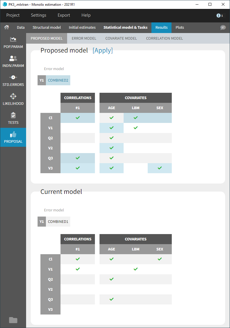
The current statistical model is displayed below the proposed model, and the differences are highlighted in light blue.
The proposed model can be applied automatically with the button “Apply”. This modifies the current project to include all elements of the proposed statistical model. It is then recommended to save the project under a new name to avoid overwriting previous results.
Error model
The error model selection is done by computing the criterion for each possible residual error model (constant, proportional, combined1, combined2), where the error parameters are optimized based on the data and the current predictions, for each observation model.
The evaluated models are displayed for each observation mode in increasing order of criterion. The current error model is highlighted in blue.
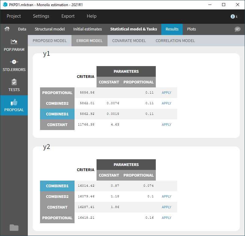
Covariate model
The covariate model selection is based on the evaluation of the criterion for each individual parameter independently.
For each individual parameter, all covariate models obtained by adding or removing one covariate are evaluated: beta parameters are estimated with linear regression, and the criterion is computed. The model with the best criterion is retained to continue the same procedure.
All evaluated models are displayed for each parameter, in increasing order of criterion. The current covariate model is highlighted in blue.
Since possibly many covariate models can be evaluated for each parameter, the maximum number of displayed models per parameter is 4 by default and can be changed with a slider, as below. Additional evaluated models can still be displayed by clicking on “more entries” below each table.
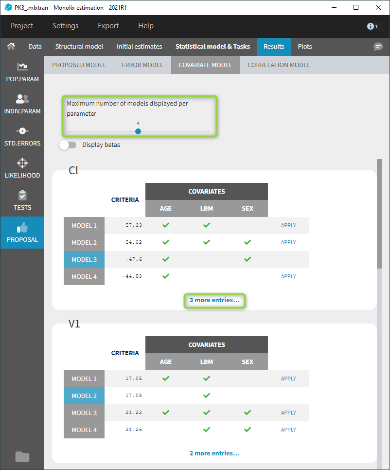
Beta parameters are computed for each evaluated model by linear regression. They are not displayed by default, but can be displayed with a toggle as shown below. For categorical covariates, the categories corresponding to the beta parameters are also displayed.
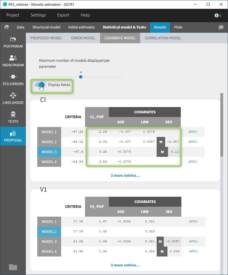
Correlation model
The correlation model selection is done by computing the criterion for each possible correlation block at each dimension, starting with the best solution from the previous dimension. The correlation models are displayed by increasing value of criterion. The current correlation model is highlighted in blue.
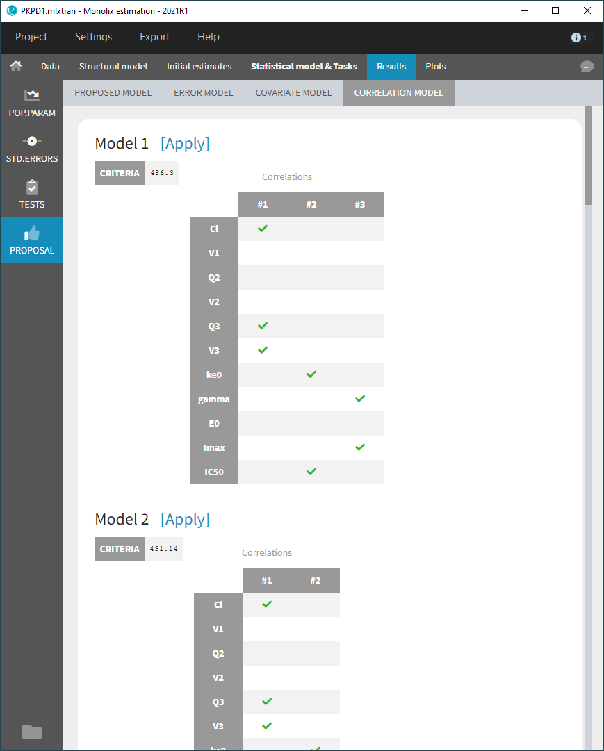
In Monolix2021, the correlation model includes also random effects at the inter-occasion level, like in the example below, while they were excluded from the proposal in previous versions.
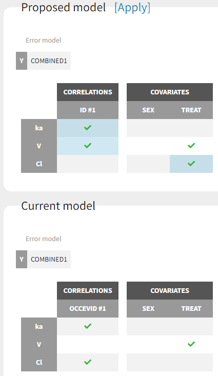
5.1.5.Standard error using the Fisher Information Matrix
- Purpose
- Calculation of the standard errors
- Running the standard errors task
- Outputs
- In the graphical user interface
- In the output folder
- Interpreting the correlation matrix of the estimates
- Settings
- Good practice
Purpose
The standard errors represent the uncertainty of the estimated population parameters. In Monolix, they are calculated via the estimation of the Fisher Information Matrix. They can for instance be used to calculate confidence intervals or detect model overparametrization.
Calculation of the standard errors
Several methods have been proposed to estimate the standard errors, such as bootstrapping or via the Fisher Information Matrix (FIM). In the Monolix GUI, the standard errors are estimated via the FIM. Bootstrapping can be accessed either through the RsSimulx R package or is now incorporated directly into the Monolix interface starting from version 2024R1.
The Fisher Information Matrix (FIM)
The observed Fisher information matrix (FIM) \(I \) is minus the second derivatives of the observed log-likelihood:
$$ I(\hat{\theta}) = -\frac{\partial^2}{\partial\theta^2}\log({\cal L}_y(\hat{\theta})) $$
The log-likelihood cannot be calculated in closed form and the same applies to the Fisher Information Matrix. Two different methods are available in Monolix for the calculation of the Fisher Information Matrix: by linearization or by stochastic approximation.
Via stochastic approximation
A stochastic approximation algorithm using a Markov chain Monte Carlo (MCMC) algorithm is implemented in Monolix for estimating the FIM. This method is extremely general
and can be used for many data and model types (continuous, categorical, time-to-event, mixtures, etc.).
Via linearization
This method can be applied for continuous data only. A continuous model can be written as:
$$\begin{array}{cl} y_{ij} &= f(t_{ij},z_i)+g(t_{ij},z_i)\epsilon_{ij} \\ z_i &= z_{pop}+\eta_i \end{array}$$
with \( y_{ij} \) the observations, f the prediction, g the error model, \( z_i\) the individual parameter value for individual i, \( z_{pop}\) the typical parameter value within the population and \(\eta_i\) the random effect.
Linearizing the model means using a Taylor expansion in order to approximate the observations \( y_{ij} \) by a normal distribution. In the formulation above, the appearance of the random variable \(\eta_i\) in the prediction f in a nonlinear way leads to a complex (non-normal) distribution for the observations \( y_{ij} \).
The Taylor expansion is done around the EBEs value, that we note \( z_i^{\textrm{mode}} \).
Standard errors
Once the Fisher Information Matrix has been obtained, the standard errors can be calculated as the square root of the diagonal elements of the inverse of the Fisher Information Matrix. The inverse of the FIM \(I(\hat{\theta})\) is the variance-covariance matrix \(C(\hat{\theta})\):
$$C(\hat{\theta})=I(\hat{\theta})^{-1}$$
The standard error for parameter \( \hat{\theta}_k \) can be calculated as:
$$\textrm{s.e}(\hat{\theta}_k)=\sqrt{\tilde{C}_{kk}(\hat{\theta})}$$
Note that in Monolix, the Fisher Information Matrix and variance-covariance matrix are calculated on the transformed normally distributed parameters. MonolixSuite version 2024R1 incorporates a change in the calculation of the variance covariance matrix \( \tilde{C} \). In version 2023 and before, \( \tilde{C} \) was obtained for untransformed parameters using the Jacobian matrix \(J\). The Jacobian matrix is a first-order approximation.
$$\tilde{C}=J^TC J$$
Starting from version 2024R1 and later, the Jacobian matrix has been replaced by exact formulas to compute the variance, dependent on the distribution of the parameters. Parameters are distingushed into those with normal distribution, lognormal distribution, as well as logit and probitnormal distribution:
- Normal distributed parameters: No transformation is required.
- Lognormal distributed parameters: The variance in the Gaussian domain (e.g variance of log(V_pop)) are obtained via the FIM. To obtain the variance of the untransformed parameyers (e.g variance of V_pop), the following formula is applied: \( Var(\hat{\theta}_{k}) = (\exp(\sigma ^{2}-1))\exp(2\mu + \sigma ^{2})\), with \( \mu = \ln(\hat{\theta}_{k}) \) and \( \sigma ^{2}=Var(\ln(\hat{\theta}_{k}))\)
- Logitnormal and probitnormal distributed parameters: There are no explicit formula to obtain the variance of the untransformed parameters (e.g bioavailability F) from the transformed parameter (e.g logit(F)). Therefore, a Monte Carlo sampling approach is used. 100000 samples are drawn from the covariance matrix in gaussian domain. Then the samples are transformed from gaussian to non-gaussian domain. For instance in the case of a logitnormal distributed parameter within bounds \( a\) and \( b\), the \(i\)-th sample of parameter \( \theta_{k,i}\): \(\mu_{k,i}=logit(\theta_{k,i})\) is transformed into non-gaussian space by the inverse logit, i.e. \(\theta_{k,i}=\frac{b \times \exp(\mu_{k,i})+ a}{(1 + \exp(\mu_{k,i}))}\). Then the empirical variance \(\sigma^2\) over all transformed samples \(\theta_{k}\) is calculated.
This transformation applies only to the typical values (fixed effects) “pop”. For the other parameters (standard deviation of the random effects “omega”, error model parameters, covariate effects “beta” and correlation parameters “corr”), we obtain directly the variance of these parameters from the FIM.
Correlation matrix
The correlation matrix is calculated from the variance-covariance matrix as:
$$\text{corr}(\theta_i,\theta_j)=\frac{\tilde{C}_{ij}}{\textrm{s.e}(\theta_i)\textrm{ s.e}(\theta_j)}$$
Wald test
For the beta parameters characterizing the influence of the covariates, the relative standard error can be used to perform a Wald test, testing if the estimated beta value is significantly different from zero.
Running the standard errors task
When running the standard error task, the progress is displayed in the pop-up window. At the end of the task, the correlation matrix is also shown, along with the elapsed time and number of iterations.
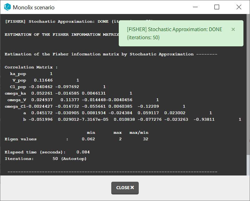
Dependencies between tasks:
The “Population parameters” task must be run before launching the Standard errors task. If the Conditional distribution task has already been run, the first iterations of the Standard errors (without linearization) will be very fast, as they will reuse the same draws as those obtained in the Conditional distribution task.
Output
In the graphical user interface
In the Pop.Param section of the Results tab, three additional columns appear in addition to the estimated population parameters:
- S.E: the estimated standard errors
- R.S.E: the relative standard error (standard error divided by the estimated parameter value)
To help the user in the interpretation, a color code is used for the p-value and the RSE:
- For the p-value: between .01 and .05, between .001 and .01, and less than .001.
- For the RSE: between 50% and 100%, between 100% and 200%, and more than 200%.
When the standard errors were estimated both with and without linearization, the S.E and R.S.E are displayed for both methods.
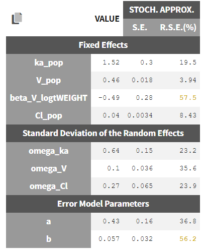
In the STD.ERRORS section of the Results tab, we display:
- R.S.E: the relative standard errors
- Correlation matrix: the correlation matrix of the population parameters
- Eigen values: the smallest and largest eigen values, as well as the condition number (max/min)
- The elapsed time and, starting from Monolix2021R1, the number of iterations for stochastic approximation, as well as a message indicating whether convergence has been reached (“auto-stop”) or if the task was stopped by the user or reached the maximum number of iterations.
To help the user in the interpretation, a color code is used:
- For the correlation: between .5 and .8, between .8 and .9, and higher than .9.
- For the RSE: between 50% and 100%, between 100% and 200%, and more than 200%.
When the standard errors were estimated both with and without linearization, both results appear in different subtabs.
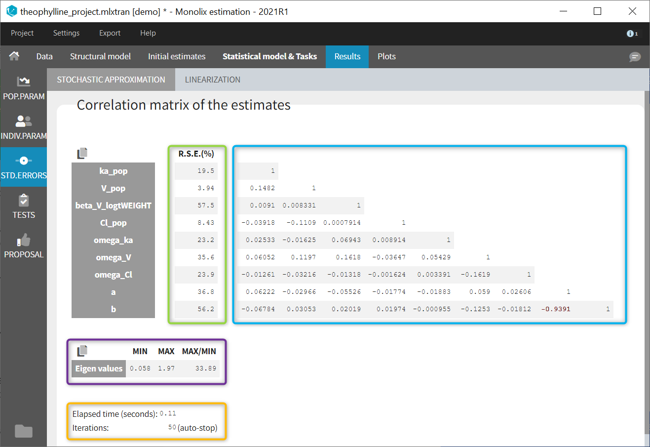
If you hover on a specific value with the mouse, both parameters are highlighted to know easily which parameter you are looking at:
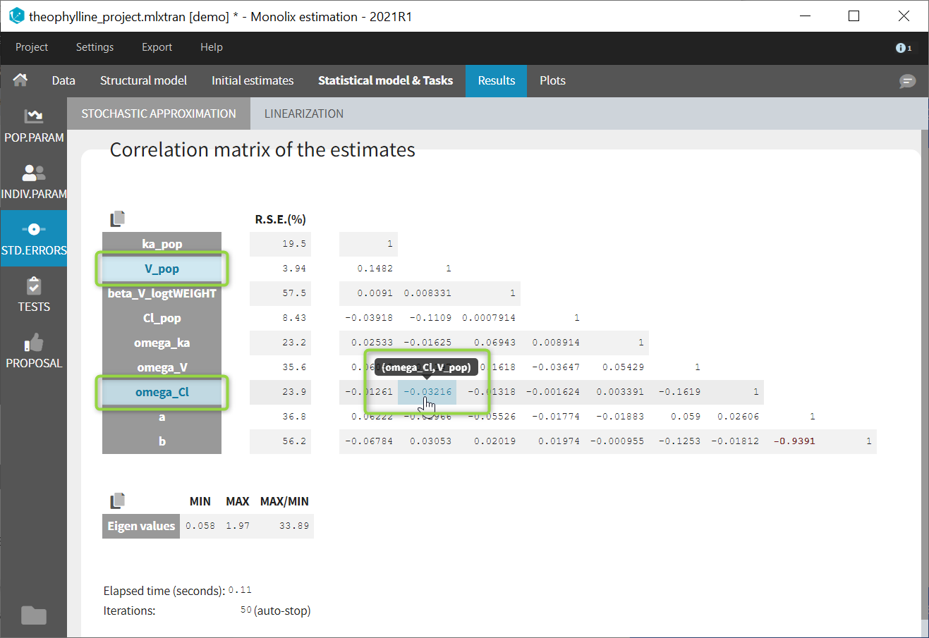
In the output folder
After having run the Standard errors task, the following files are available:
- summary.txt: contains the s.e, r.s.e, p-values, correlation matrix and eigenvalues in an easily readable format, as well as elapsed time and number of iterations for stochastic approximation (starting from Monolix2021R1).
- populationParameters.txt: contains the s.e, r.s.e and p-values in csv format, for the method with (*_lin) or without (*_sa) linearization
- FisherInformation/correlationEstimatesSA.txt: correlation matrix of the population parameter estimates, method without linearization (stochastic approximation)
- FisherInformation/correlationEstimatesLin.txt: correlation matrix of the population parameter estimates, method with linearization
- FisherInformation/covarianceEstimatesSA.txt: variance-covariance matrix of the transformed normally distributed population parameter, method without linearization (stochastic approximation)
- FisherInformation/covarianceEstimatesLin.txt: variance-covariance matrix of the transformed normally distributed population parameter, method with linearization
Interpreting the correlation matrix of the estimates
The color code of Monolix’s results allows to quickly identify population parameter estimates that are strongly correlated. This often reflects model overparameterization and can be further investigated using Mlxplore and the convergence assessment. This is explained in details in this video:
Settings
The settings are accessible through the interface via the button next to the Standard errors task:

- Minimum number of iterations: minimum number of iterations of the stochastic approximation algorithm to calculate the Fisher Information Matrix.
- Maximum number of iterations: maximum number of iterations of the stochastic approximation algorithm to calculate the Fisher Information Matrix. The algorithm stops even if the stopping criteria are not met.
Good practices and tips
When to use “use linearization method”?
Firstly, it is only possible to use the linearization method for continuous data. For the linearization is available, this method is generally much faster than without linearization (i.e stochastic approximation) but less precise. The Fisher Information Matrix by model linearization will generally be able to identify the main features of the model. More precise– and time-consuming – estimation procedures such as stochastic approximation will have very limited impact in terms of decisions for these most obvious features. Precise results are required for the final runs where it becomes more important to rigorously defend decisions made to choose the final model and provide precise estimates and diagnosis plots.
I have NANs as results for standard errors for parameter estimates. What should I do? Does it impact the likelihood?
NaNs as standard errors often appear when the model is too complex and some parameters are unidentifiable. They can be seen as an infinitely large standard error.
The likelihood is not affected by NaNs in the standard errors. The estimated population parameters having a NaN as standard error are only very uncertain (infinitely large standard error and thus infinitely large confidence intervals).
5.1.6.Log Likelihood estimation
Purpose
The log-likelihood is the objective function and a key information. The log-likelihood cannot be computed in closed form for nonlinear mixed effects models. It can however be estimated.
Log-likelihood estimation
Performing likelihood ratio tests and computing information criteria for a given model requires computation of the log-likelihood
$$ {\cal L}{\cal L}_y(\hat{\theta}) = \log({\cal L}_y(\hat{\theta})) \triangleq \log(p(y;\hat{\theta})) $$
where \(\hat{\theta}\) is the vector of population parameter estimates for the model being considered, and \(p(y;\hat{\theta})\) is the probability distribution function of the observed data given the population parameter estimates. The log-likelihood cannot be computed in closed form for nonlinear mixed effects models. It can however be estimated in a general framework for all kinds of data and models using the importance sampling Monte Carlo method. This method has the advantage of providing an unbiased estimate of the log-likelihood – even for nonlinear models – whose variance can be controlled by the Monte Carlo size.
Two different algorithms are proposed to estimate the log-likelihood:
- by linearization,
- by Importance sampling.
Log-likelihood by importance sampling
The observed log-likelihood \({\cal LL}(\theta;y)=\log({\cal L}(\theta;y))\) can be estimated without requiring approximation of the model, using a Monte Carlo approach. Since
$${\cal LL}(\theta;y) = \log(p(y;\theta)) = \sum_{i=1}^{N} \log(p (y_i;\theta))$$
we can estimate \(\log(p(y_i;\theta))\) for each individual and derive an estimate of the log-likelihood as the sum of these individual log-likelihoods. We will now explain how to estimate \(\log(p(y_i;\theta))\) for any individual i. Using the \(\phi\)-representation of the model (the individual parameters are transformed to be Gaussian), notice first that \(p(y_i;\theta)\) can be decomposed as follows:
$$p(y_i;\theta) = \int p(y_i,\phi_i;\theta)d\phi_i = \int p(y_i|\phi_i;\theta)p(\phi_i;\theta)d\phi_i = \mathbb{E}_{p_{\phi_i}}\left(p(y_i|\phi_i;\theta)\right)$$
Thus, \(p(y_i;\theta)\) is expressed as a mean. It can therefore be approximated by an empirical mean using a Monte Carlo procedure:
- Draw M independent values \(\phi_i^{(1)}\), \(\phi_i^{(2)}\), …, \(\phi_i^{(M)}\) from the marginal distribution \(p_{\phi_i}(.;\theta)\).
- Estimate \(p(y_i;\theta)\) with \(\hat{p}_{i,M}=\frac{1}{M}\sum_{m=1}^{M}p(y_i | \phi_i^{(m)};\theta)\)
By construction, this estimator is unbiased, and consistent since its variance decreases as 1/M:
$$\mathbb{E}\left(\hat{p}_{i,M}\right)=\mathbb{E}_{p_{\phi_i}}\left(p(y_i|\phi_i^{(m)};\theta)\right) = p(y_i;\theta) ~~~~\mbox{Var}\left(\hat{p}_{i,M}\right) = \frac{1}{M} \mbox{Var}_{p_{\phi_i}}\left(p(y_i|\phi_i^{(m)};\theta)\right)$$
We could consider ourselves satisfied with this estimator since we “only” have to select M large enough to get an estimator with a small variance. Nevertheless, it is possible to improve the statistical properties of this estimator.
For any distribution \(\tilde{p_{\phi_i}}\) that is absolutely continuous with respect to the marginal distribution \(p_{\phi_i}\), we can write
$$ p(y_i;\theta) = \int p(y_i|\phi_i;\theta) \frac{p(\phi_i;\theta)}{\tilde{p}(\phi_i;\theta)} \tilde{p}(\phi_i;\theta)d\phi_i = \mathbb{E}_{\tilde{p}_{\phi_i}}\left(p(y_i|\phi_i;\theta)\frac{p(\phi_i;\theta)}{\tilde{p}(\phi_i;\theta)} \right).$$
We can now approximate \(p(y_i;\theta)\) using an importance sampling integration method with \(\tilde{p}_{\phi_i}\) as the proposal distribution:
- Draw M independent values \(\phi_i^{(1)}\), \(\phi_i^{(2)}\), …, \(\phi_i^{(M)}\) from the proposal distribution \(\tilde{p_{\phi_i}}(.;\theta)\).
- Estimate \(p(y_i;\theta)\) with \(\hat{p}_{i,M}=\frac{1}{M}\sum_{m=1}^{M}p(y_i | \phi_i^{(m)};\theta)\frac{p(\phi_i^{(m)};\theta)}{\tilde{p}(\phi_i^{(m)};\theta)}\)
By construction, this estimator is unbiased, and its variance also decreases as 1/M:
$$\mbox{Var}\left(\hat{p}_{i,M}\right) = \frac{1}{M} \mbox{Var}_{\tilde{p_{\phi_i}}}\left(p(y_i|\phi_i^{(m)};\theta)\frac{p(\phi_i^{(m)};\theta)}{\tilde{p}(\phi_i^{(m)};\theta)}\right)$$
There exist an infinite number of possible proposal distributions \(\tilde{p}\) which all provide the same rate of convergence 1/M. The trick is to reduce the variance of the estimator by selecting a proposal distribution so that the numerator is as small as possible.
For this purpose, an optimal proposal distribution would be the conditional distribution \(p_{\phi_i|y_i}\). Indeed, for any \(m = 1,2, …, M,\)
$$ p(y_i|\phi_i^{(m)};\theta)\frac{p(\phi_i^{(m)};\theta)}{p(\phi_i^{(m)}|y_i;\theta)} = p(y_i;\theta) $$
which has a zero variance, so that only one draw from \(p_{\phi_i|y_i}\) is required to exactly compute the likelihood \(p(y_i;\theta)\).
The problem is that it is not possible to generate the \(\phi_i^{(m)}\) with this exact conditional distribution, since that would require computing a normalizing constant, which here is precisely \(p(y_i;\theta)\).
Nevertheless, this conditional distribution can be estimated using the Metropolis-Hastings algorithm and a practical proposal “close” to the optimal proposal \(p_{\phi_i|y_i}\) can be derived. We can then expect to get a very accurate estimate with a relatively small Monte Carlo size M.
The mean and variance of the conditional distribution \(p_{\phi_i|y_i}\) are estimated by Metropolis-Hastings for each individual i. Then, the \(\phi_i^{(m)}\) are drawn with a noncentral student t-distribution:
$$ \phi_i^{(m)} = \mu_i + \sigma_i \times T_{i,m}$$
where \(\mu_i\) and \(\sigma^2_i\) are estimates of \(\mathbb{E}\left(\phi_i|y_i;\theta\right)\) and \(\mbox{Var}\left(\phi_i|y_i;\theta\right)\), and \((T_{i,m})\) is a sequence of i.i.d. random variables distributed with a Student’s t-distribution with \(\nu\) degrees of freedom (see section Advanced settings for the log-likelihood for the number of degrees of freedom).
Remark: The standard error of the LL on all the draws is proposed. It represents the impact of the variability of the draws on the LL uncertainty, given the estimated population parameters, but it does not take into account the uncertainty of the model that comes from the uncertainty on the population parameters.
Remark: Even if \(\hat{\cal L}_y(\theta)=\prod_{i=1}^{N}\hat{p}_{i,M}\) is an unbiased estimator of \({\cal L}_y(\theta)\), \(\hat{\cal LL}_y(\theta)\) is a biased estimator of \({\cal LL}_y(\theta)\). Indeed, by Jensen’s inequality, we have :
$$\mathbb{E}\left(\log(\hat{\cal L}_y(\theta))\right) \leq \log \left(\mathbb{E}\left(\hat{\cal L}_y(\theta)\right)\right)=\log\left({\cal L}_y(\theta)\right)$$
Best practice: the bias decreases as M increases and also if \(\hat{\cal L}_y(\theta)\) is close to \({\cal L}_y(\theta)\). It is therefore highly recommended to use a proposal as close as possible to the conditional distribution \(p_{\phi_i|y_i}\), which means having to estimate this conditional distribution before estimating the log-likelihood (i.e. run task “Conditional distribution” before).
Log-likelihood by linearization
The likelihood of the nonlinear mixed effects model cannot be computed in a closed-form. An alternative is to approximate this likelihood by the likelihood of the Gaussian model deduced from the nonlinear mixed effects model after linearization of the function f (defining the structural model) around the predictions of the individual parameters \((\phi_i; 1 \leq i \leq N)\).
Notice that the log-likelihood can not be computed by linearization for discrete outputs (categorical, count, etc.) nor for mixture models.
Best practice: We strongly recommend to compute the conditional mode before computing the log-likelihood by linearization. Indeed, the linearization should be made around the most probable values as they are the same for both the linear and the nonlinear model.
Best practices: When should I use the linearization and when should I use the importance sampling?
Firstly, it is only possible to use the linearization algorithm for the continuous data. In that case, this method is generally much faster than importance sampling method and also gives good estimates of the LL. The LL calculation by model linearization will generally be able to identify the main features of the model. More precise– and time-consuming – estimation procedures such as stochastic approximation and importance sampling will have very limited impact in terms of decisions for these most obvious features. Selection of the final model should instead use the unbiased estimator obtained by Monte Carlo.
Display and outputs
In case of estimation using the importance sampling method, a graphical representation is proposed to see the valuation of the mean value over the Monte Carlo iterations as on the following:
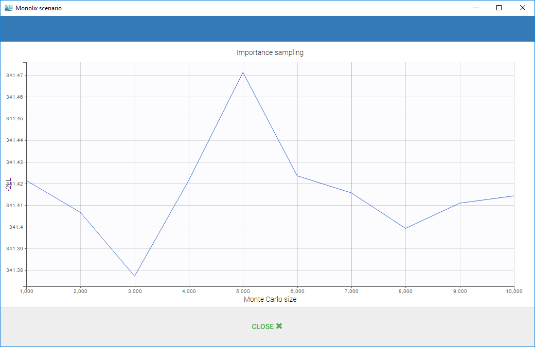
The final estimations are displayed in the result frame as below. Notice that there is a “Copy table” icon on the top of each table to copy them in Excel, Word, … The table format and display will be kept.
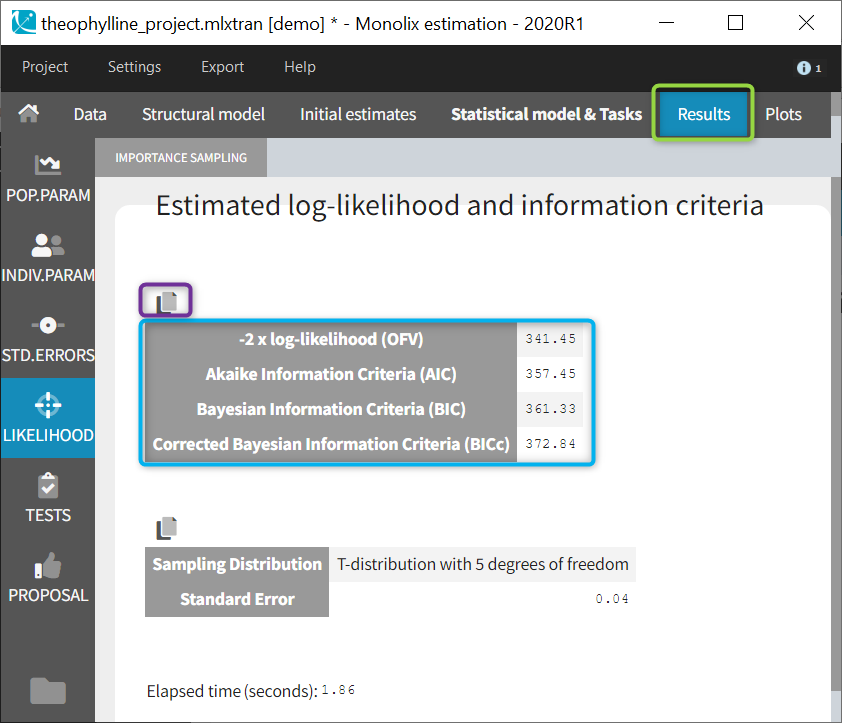
The log-likelihood is given in Monolix together with the Akaike information criterion (AIC) and Bayesian information criterion (BIC):
$$ AIC = -2 {\cal L}{\cal L}_y(\hat{\theta}) +2P $$
$$ BIC = -2 {\cal L}{\cal L}_y(\hat{\theta}) +log(N)P $$
where P is the total number of parameters to be estimated and N the number of subjects.
The new BIC criterion penalizes the size of \(\theta_R\) (which represents random effects and fixed covariate effects involved in a random model for individual parameters) with the log of the number of subjects (\(N\)) and the size of \(\theta_F\) (which represents all other fixed effects, so typical values for parameters in the population, beta parameters involved in a non-random model for individual parameters, as well as error parameters) with the log of the total number of observations (\(n_{tot}\)), as follows:
$$ BIC_c = -2 {\cal L}{\cal L}_y(\hat{\theta}) + \dim(\theta_R)\log N+\dim(\theta_F)\log n_{tot}$$
If the log-likelihood has been computed by importance sampling, the number of degrees of freedom used for the proposal t-distribution (5 by default) is also displayed, together with the standard error of the LL on the individual parameters drawn from the t-distribution.
In terms of output, a folder called LogLikelihood is created in the result folder where the following files are created
- logLikelihood.txt: containing for each computed method, the -2 x log-likelihood, the Akaike Information Criteria (AIC), the Bayesian Information Criteria (BIC), and the corrected Bayesian Information Criteria (BICc).
- individualLL.txt: containing the -2 x log-likelihood for each individual for each computed method.
Advanced settings for the log-likelihood
Monolix uses a t-distribution as proposal. By default, the number of degrees of freedom of this distribution is fixed to 5. In the settings of the task, it is also possible to optimize the number of degrees of freedom. In such a case, the default possible values are 1, 2, 5, 10 and 20 degrees of freedom. A distribution with a small number of degree of freedom (i.e. heavy tails) should be avoided in case of stiff ODE’s defined models.
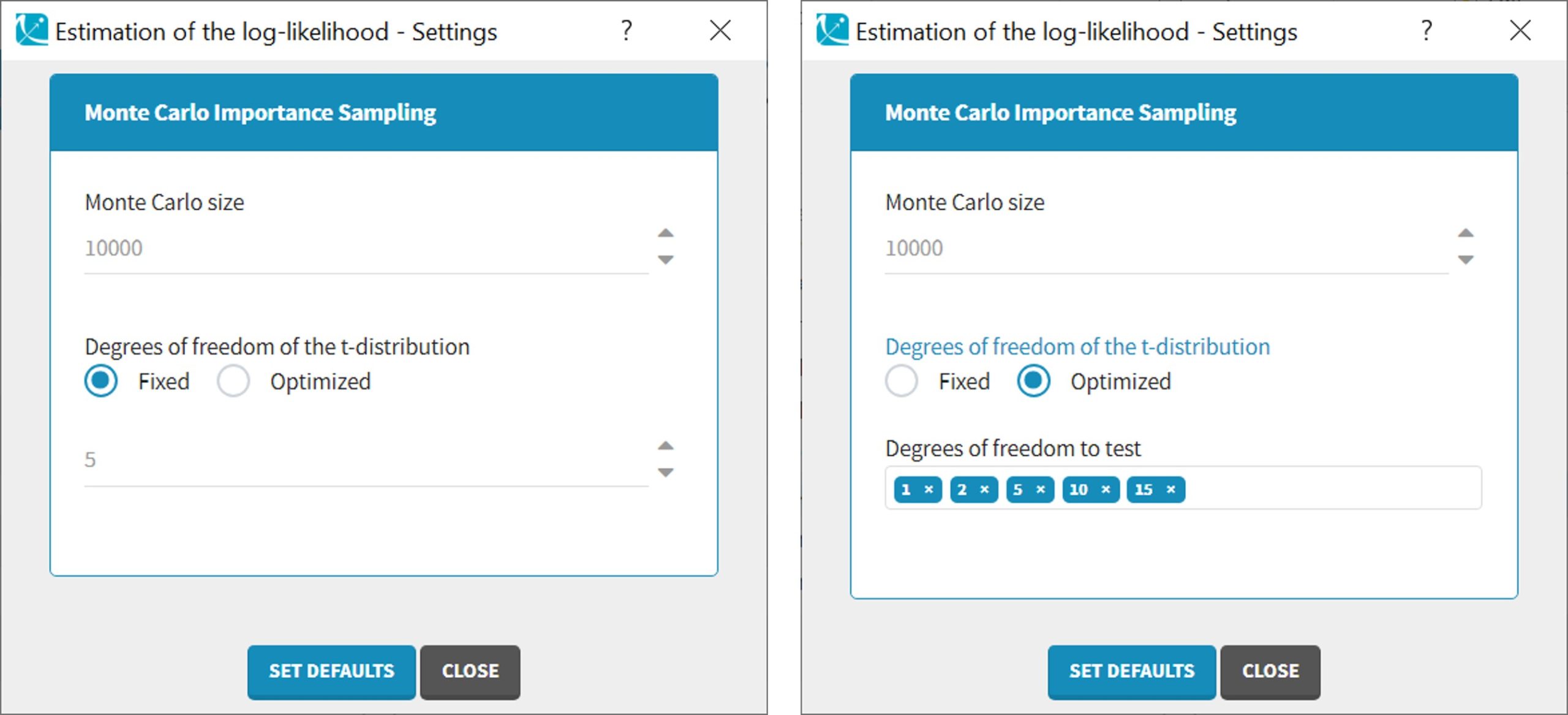
5.2.Algorithms convergence assessment
Monolix includes a convergence assessment tool. It allows to execute a workflow of estimation tasks several times, with different, randomly generated, initial values of fixed effects, as well as different seeds. The goal is to assess the robustness of the convergence.
Running the convergence assessment
For that, click on the shortcut button in the “Tasks” part.
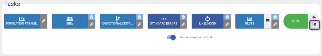
A dedicated panel opens as in the figure below. The first shortcut button next to Run can be used to go back to the estimation.
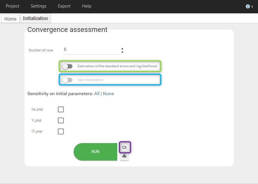
The user can define
-
- the number of runs, or replicates
- the type of assessment:
- Estimation of the standard errors and log-likelihood
- Use the linearization method if the previous option is selected.
- the initial parameters. By default, initial values are uniformly drawn from intervals defined around the estimated values if population parameters have been estimated, the initial estimates otherwise. Notice that it is possible to set one initial parameter constant while generating the others. The minimum and maximum of the generated parameters can be modified by the user.
All settings used are saved and reloaded with the run containing the convergence assessment results.
Notice that
- In the case of estimation of the standard errors and log-likelihood by linearization, the individual parameters with the conditional mode method are computed as well to have more relevant linearization.
- In the case of estimation of the standard errors and log-likelihood without the linearization, the conditional distribution method is computed too to have more relevant estimation.
- The workflow is the same between the runs and is not the one defined in the interface.
Click on Run to execute the tool. Thus you are able to estimate the population parameters using several initial seeds and/or several initial conditions.
Display and outputs
Several kinds of plots are given as a summary of the results.
First of all, the SAEM convergence assessment is proposed. The convergence of each parameter on each run is proposed. It allows to see if the convergence for each run is ok.
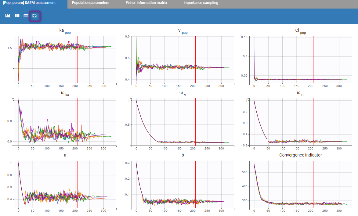
Then, a plot showing the estimated values for each replicate is proposed. If the estimation of the standard errors was included in the scenario, the estimated standard errors are also displayed as horizontal bars. It allows to see if all parameters converge statistically to the same values.
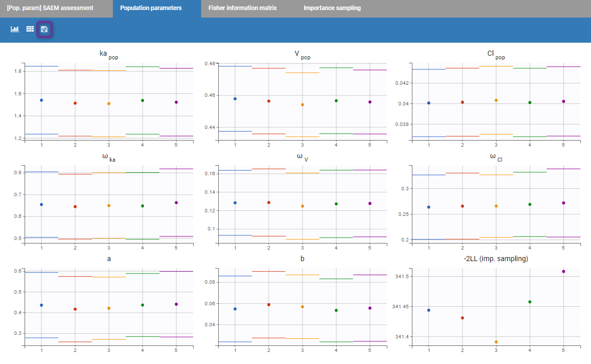
Starting from the 2019 version, it is possible to export manually all the plots in the Assessment folder in your result folder by clicking on the “export” icon (purple box on the previous figure).
Finally, if log-likelihood without linearization is used, the curves for convergence of importance sampling are proposed.
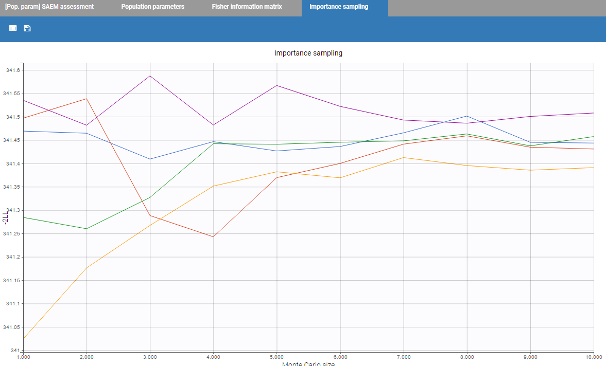
In addition, a Monolix project and its result folder is generated for each set of initial parameters. They are located in the Assessment subfolder of the main project’s result folder (located by default next to the .mlxtran project file). Along with all the runs, there is a summary of all the runs “assessment.txt” providing all the individual parameter estimates along with the -2LL, as in the following:
Parameters,Run_1,Run_2,Run_3,Run_4,Run_5
Cl_pop,0.03994527,0.04017999,0.04016216,0.04012077,0.0400175
V_pop,0.4575748,0.4556463,0.4560732,0.4557009,0.4569431
a,0.4239969,0.42482,0.4227559,0.4294611,0.435585
b,0.05653124,0.05684357,0.05700663,0.054965,0.05450724
ka_pop,1.527947,1.521184,1.5226,1.519333,1.519678
omega_Cl,0.2653109,0.2643172,0.268475,0.266199,0.2693083
omega_V,0.1293328,0.1274441,0.122951,0.1301242,0.1261098
omega_ka,0.6530206,0.6655251,0.643456,0.6425528,0.6424614
-2LL,339.387,339.417,339.429,339.444,339.462
Notice that, starting from the 2019 version, it is possible to reload all the results of a previous convergence if nothing has changed in the project. Starting from version 2021, the settings of the convergence assessment are also reloaded.
Best practices: what is the use the convergence assessment tool?
We cannot claim that SAEM always converges (i.e., with probability 1) to the global maximum of the likelihood. We can only say that it converges under quite general hypotheses to a maximum – global or perhaps local – of the likelihood. A large number of simulation studies have shown that SAEM converges with high probability to a “good” solution – hopefully the global maximum – after a small number of iterations. The purpose of this tool is to evaluate the SAEM algorithm with initial conditions and see if the estimated parameters are the “global” minimum.
The trajectory of the outputs of SAEM depends on the sequence of random numbers used by the algorithm. This sequence is entirely determined by the “seed.” In this way, two runs of SAEM using the same seed will produce exactly the same results. If different seeds are used, the trajectories will be different but convergence occurs to the same solution under quite general hypotheses. However, if the trajectories converge to different solutions, that does not mean that any of these results are “false”. It just means that the model is sensitive to the seed or to the initial conditions. The purpose of this tool is to evaluate the SAEM algorithm with several seeds to see the robustness of the convergence.
5.3.Model building
Starting from the 2019 version, a panel Model building provides automatic model building tools:
This panel is accessible via the button Model building next to Run in the interface of Monolix, or from the section Perspective in the tab Home.
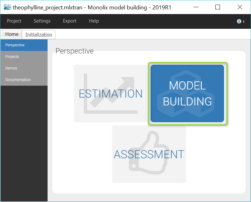 |
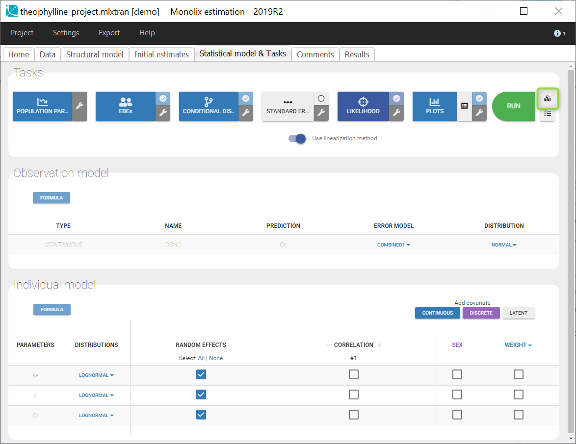 |
5.3.1.Statistical tests for model assessment
5.3.2.Automatic statistical model building (covariate model, correlation model, error model)
5.3.3.Automatic complete statistical model building
5.3.4.Automatic covariate model building
5.3.5.Automatic variability model building
5.3.6.Statistical model building with SAMBA
Starting from the 2019 version, an automatic statistical model building algorithm is implemented in Monolix: SAMBA (Stochastic Approximation for Model Building Algorithm)
SAMBA is an iterative procedure to accelerate and optimize the process of model building by identifying at each step how best to improve some of the model components (residual error model, covariate effects, correlations between random effects). This method allows to find the optimal statistical model which minimizes some information criterion in very few steps. It is described in more details in the following publication:
At each iteration, the best statistical model is selected with the same method as the Proposal. This step is very quick as it does not require to estimate new parameters with SAEM for all evaluated models. Initial estimates are set to the estimated values from the Proposal.
The population parameters of the selected model are then estimated with SAEM, individual parameters are simulated from the conditional distributions, and the log-likelihood is computed to evaluate the improvement of the model. The algorithm stops when no improvement is brought by the selected model or if it has already been tested.
Initialization
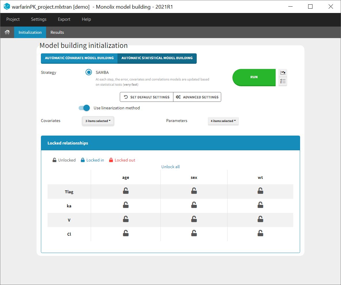
Settings
The linearization method is selected by default to compute the log-likelihood of the estimated model at each iteration. It can be unselected to use importance sampling.
The improvement can be evaluated with two different criteria based on the log-likelihood, that can be selected in the settings (available via the icon next to Run):
- BICc (by default)
- LRT (likelihood ratio threshold): by default the forward threshold is 0.01 and the backward threshold is 0.01. These values can be changed in the settings.
Starting from the 2021 version, all settings used are saved and reloaded with the run containing the model building results.
Selecting covariates and parameters
It is possible to select part of the covariates and individual parameters to be used in the algorithm:

Moreover, a panel “Locked relationships” can be opened to lock in or lock out some covariate-parameter relationships among the ones that are available:
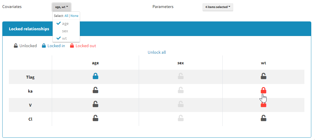
Starting from the 2021 version, all relationships considered in model building are part of the settings which are saved and reloaded with the run containing the model building results.
Results
The results of the model building are displayed in a tab Results, with the list of model run at each iteration (see for example the figure below) and the corresponding -2LL and BICc values.
All resulting runs are also located in the ModelBuilding subfolder of the project’s result folder (located by default next to the .mlxtran project file).
In the Results tab, by default runs are displayed by order of iteration, except the best model which is displayed in first position, highlighted in blue.
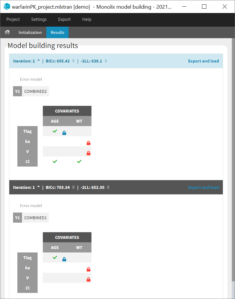
Note that the table of iterations can be sorted by iteration number or criteria (see green marks below). Buttons “export and load” (see blue mark below) can also be used to export the model estimated at this iteration as a new Monolix project with a new name and open it in the current Monolix session.
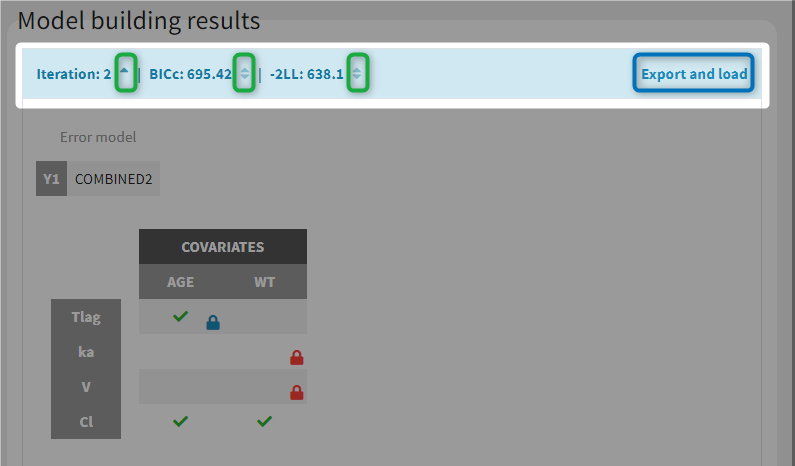
While the algorithm is running, the progress of the estimation tasks at each iteration is displayed on a white pop-up window, and temporary green messages confirm each successful task.
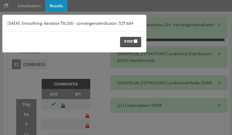
5.4.Bootstrap
[Bootstrap is not available in versions prior to 2024R1]
Introduction
The Bootstrap module in Monolix provides a robust method to assess parameter uncertainty, offering an alternative to calculating standard errors via inversion of the Fisher Information Matrix. This approach becomes particularly valuable when facing issues such as NaNs in standard errors due to numerical errors in matrix inversion or biases in results caused by incorrect assumptions of asymptotic normality for parameter estimates. Bootstrap overcomes these challenges by sampling many replicate datasets and re-estimating parameters on each replicate.
While powerful, bootstrap comes with certain drawbacks:
- Running many replicates for population parameter estimation can be time-consuming. Bootstrap in Monolix can be used from command line and with distributed calculation (parallelization on a grid via MPI).
- Saving a large number of new datasets and results may raise storage issues. You can choose in the settings whether to save sampled datasets and results.
Accessing the bootstrap module
Bootstrap can be accessed under the “Perspective” menu or with a shortcut next to “Run” in the “Statistical model & Tasks” tab:
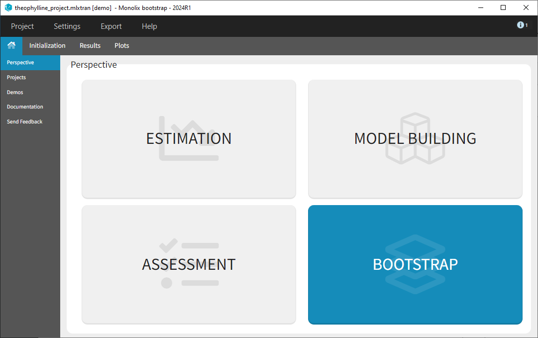
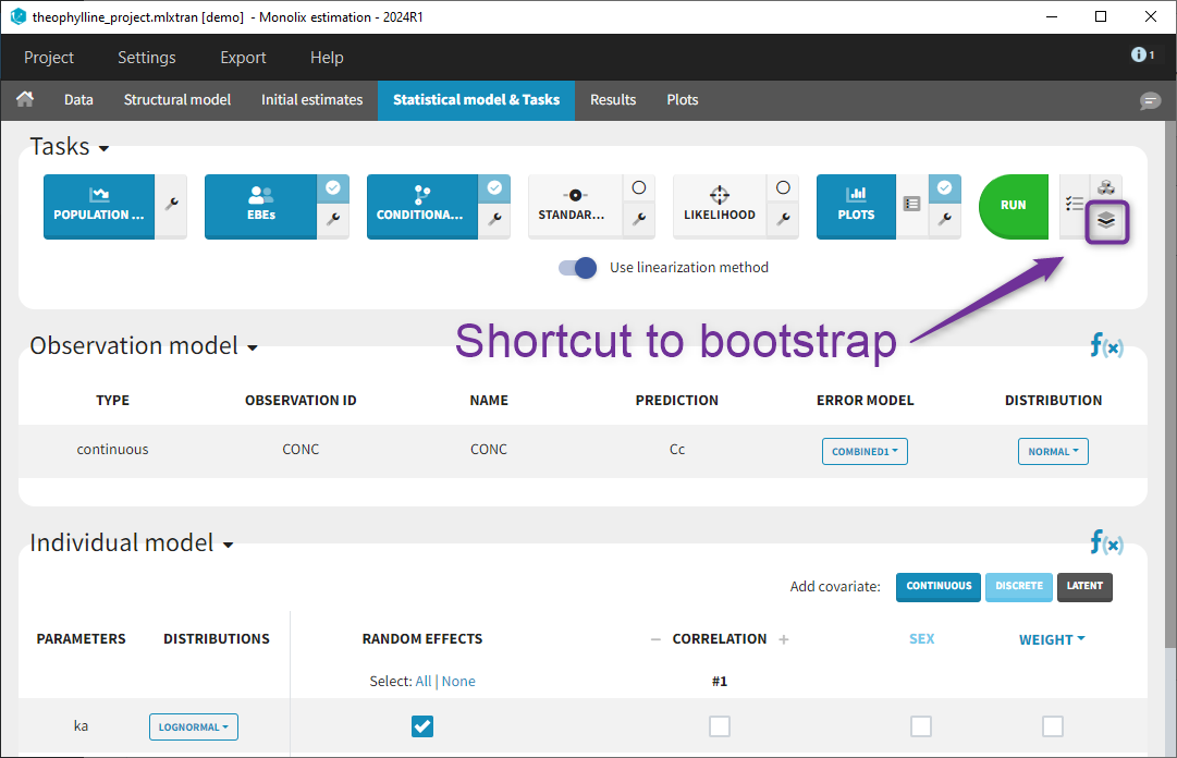
Available bootstrap settings
Users can customize the following settings:
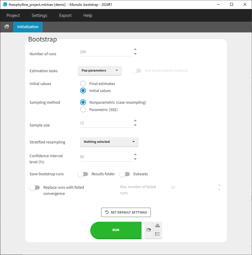
- Number of runs: Number of bootstrap replicates
- Estimation tasks: Estimation tasks to run among population pramaters, Standard Errors, and Log-Likelihood
- Initial values: Whether bootstrap runs should start their estimation from the same initial values as the initial run, or from the final estimated values from the initial run.
- Sampling method: Type of bootstrap:
- Nonparametric Bootstrap (case resampling): New datasets are sampled from the initial dataset for each replicate. Each individual of the new dataset is sampled randomly with replacement from the initial dataset. This means that some individuals from the original dataset will appear several times in the resampled dataset, while some individuals will not appear at all. The generated datasets are thus similar but different compared to the original dataset. This method makes no assumption on the model.
- Parametric Bootstrap (SSE): This method is also called SSE for stochastic simulation and estimation. New datasets are simulated from the model for each replicate. Individual parameters are sampled from the population distribution and individuals are simulated using the same design as in the original dataset (same treatments, covariates, regressors, and observation times). Residual error is added on top of the model predictions to obtain a realistic dataset. If the initial dataset has censored data, censoring limits to apply to the simulated datasets can be specified by the user. This method assumes that the model correctly captures the original data.
- Sample size: Number of individuals in the bootstrap datasets. By default it is set equal to the number of individuals of the original dataset but can be modified if required.
- Stratified resampling: Selection of categorical covariates which distribution should be preserved when re-sampling individuals to create datasets for non-parametric bootstrap. When the original dataset contains few individuals, or when a categorical covariate distribution is highly imbalanced with only few individuals belonging to one of the categories, resampled bootstrap datasets can results in quite different distributions (e.g only one individual left in one of the categories) and this can lead to a bias, in particular on the covariate effects (beta) parameters. To avoid this situation, the sampling can be done such that the number of individuals in each category of the covariates selected in “stratified resampling” remains the same as in the initial dataset.
- Confidence interval level: Level of the confidence interval bounds displayed in the results to summarize the uncertainty on the population parameters.
- Save bootstrap runs: Option to save or not save bootstrap datasets and results folder of each bootstrap run. Both options need to be selected if you want to be able to reload each bootstrap run including the results.
- Replace runs with failed convergence: Option to replace or not bootstrap replicates that have a failed convergence. This option allows to replace runs for which the “auto-stop” criteria of the exploratiry phase of the population parameter estimation have not been reached. You can also set a maximal number of runs to replace, so that bootstrap will not go on forever if many runs do not converge. Bootstrap will stop once the maximal number is reached.
Running bootstrap
After clicking on “Run”, bootstrap is launched and the population parameters estimates from all runs already done are shown as a table and as a plot of their medians and their confidence intervals with respect to the bootstrap iterations. The table and plot updates as soon as new bootstrap run finishes. An estimation of the remaining time to complete all bootstrap runs is available at the top.
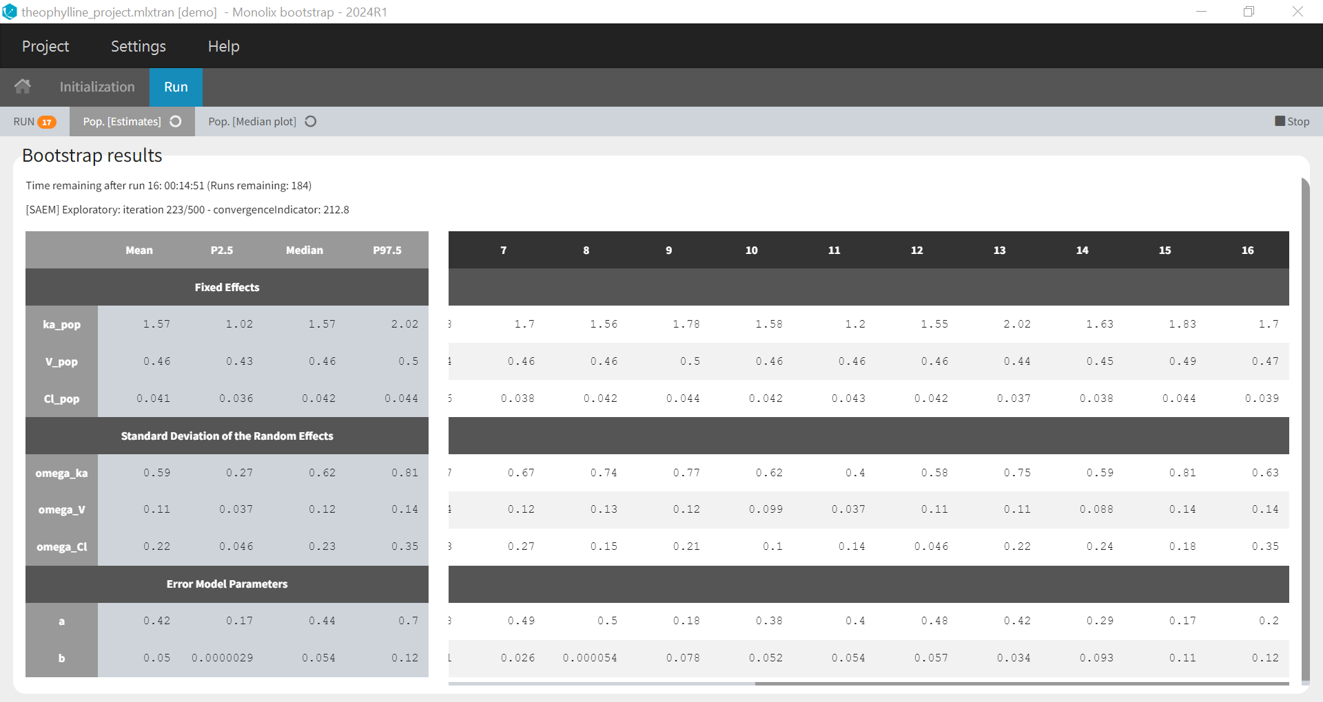
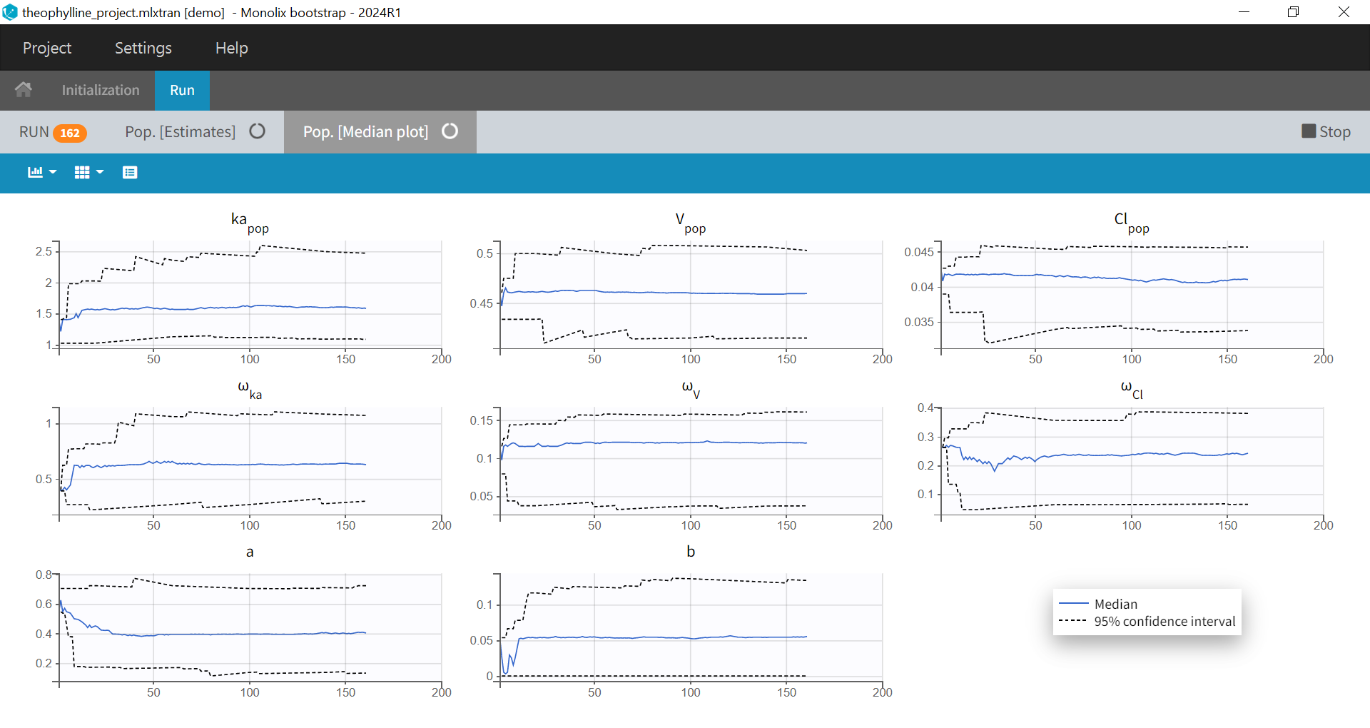
If you have stopped bootstrap before the last run, or you want to add more runs to your bootstrap results, you can resume bootstrap so that the runs already done will be reused instead of being rerun:

Results
Bootstrap results reported in the interface and the output files include the following. Depending on the choice of estimation tasks in the bootstrap settings, results for population parameters, RSE (if Standard error task was selected), and LL (if log-likelihood task was selected) are available.
- Results > [Estimates]: Estimates from each bootstrap run displayed in tables.
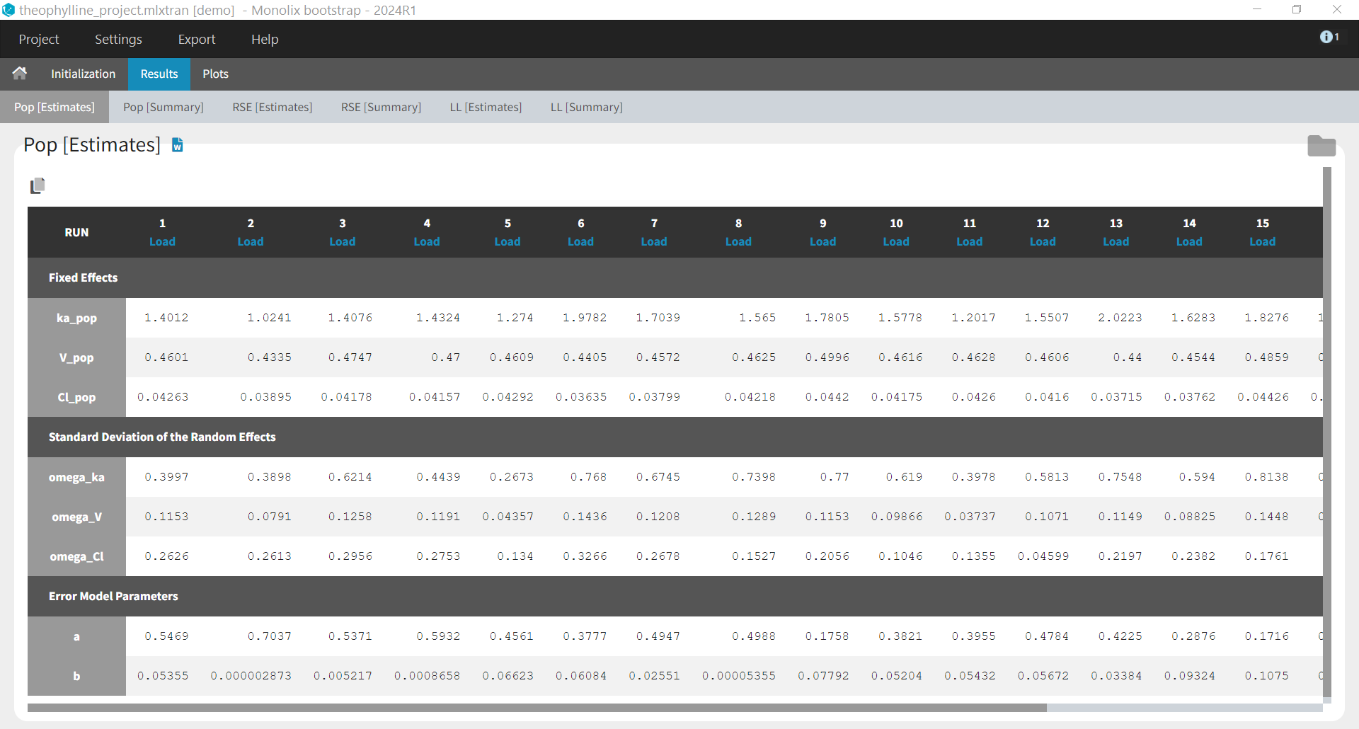
When the options to save both the results folder and the datasets have been selected, it is possible to load each bootstrap run via the “load” button in the “Pop [Estimates]” tab:
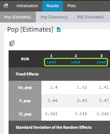
- Plots: Estimates from each bootstrap run displayed as distribution plots. Distribution plots can be displayed as boxplots or as histogramms (pdf).
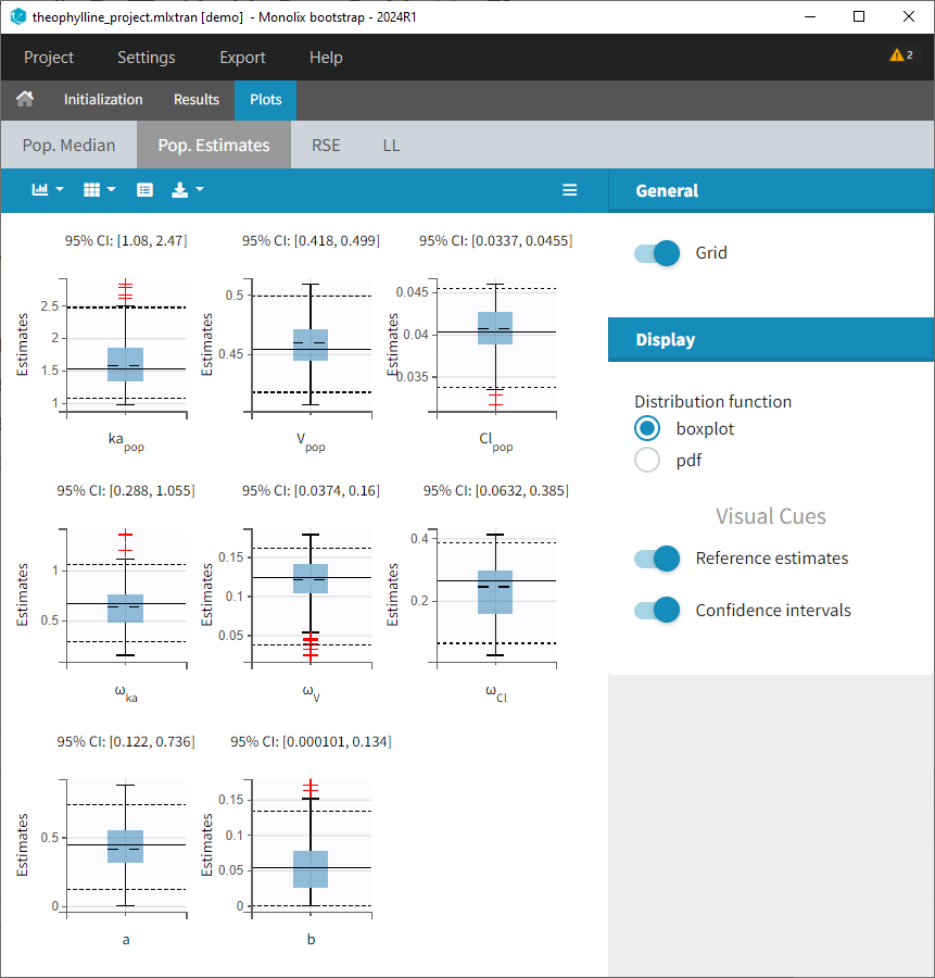
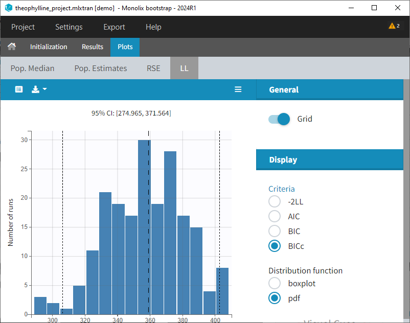
- Results > [Summary]: Summary table of bootstrap estimates including value of the initial run (reference), mean and median over bootstrap runs, standard error (SE) over bootstrap runs, relative standard error (RSE) over bootstrap runs, confidence intervals (according to chosen confidence level). For population parameter, the bias of the mean over bootstrap runs compared ot the reference value is calculated as bias = (mean – reference)/reference*100.
If some runs have not reached convergences, a toggle appears to filter the summary table and keep only runs which have converged.
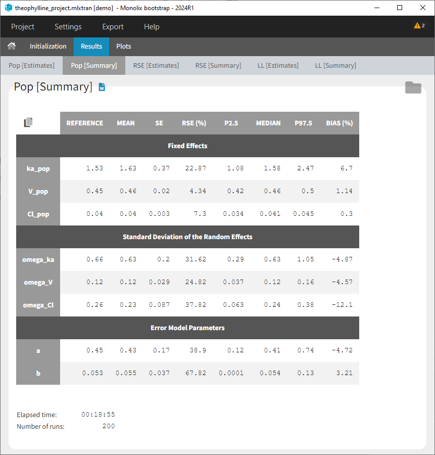
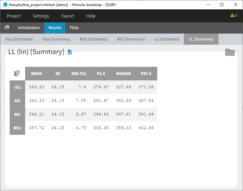
- Main window (Estimation) > Results > Pop Param: The bootstrap results also appear in the table of population parameter estimates of the parent run. This is convenient to compare the estimated values and their confidence intervals estimated via the Fisher Information Matrix, to the median and confidence intervals estimated via bootstrap. Bootstrap results can be included in the pop param table when generating reports from Monolix.
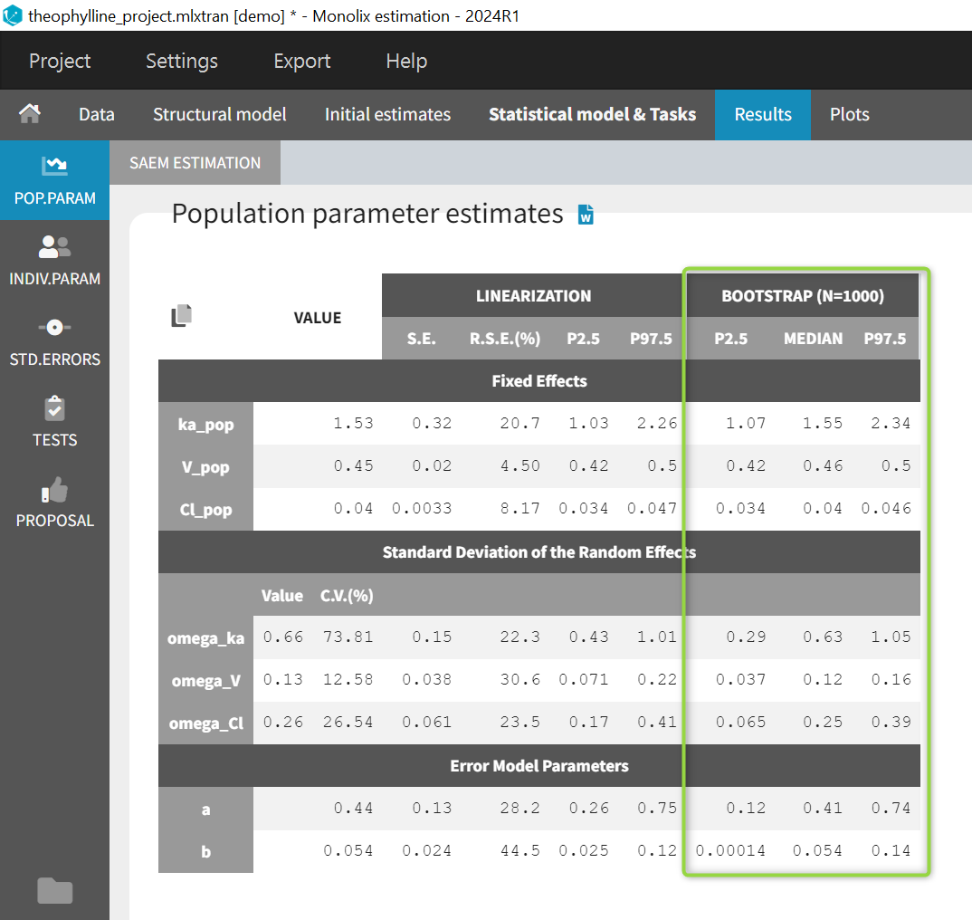
- Saved datasets: In the case of non-parametric bootstrap, resampled datasets used in bootstrap runs have new subject identifiers defined as integers in the column tagged as ID, and include an additional column named “original_id” with the corresponding subject identifiers from the initial dataset.
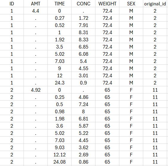
5.5.Output files
Monolix generates a lot of different output files depending on the tasks done by the user. Here is a complete listing of the files, along with the condition for their creation and their content.
- Task: Population parameter estimation
- Task: Individual parameter estimation
- Task: Fisher Information Matrix calculation
- Task: Log-likelihood calculation
- Tests
- Tables
- ChartsData
Population parameter estimation
summary.txt
Description: summary file.
Outputs:
- Header: project file name, date and time of run, Monolix version
- Estimation of the population parameters: Estimated population parameters & computation time
populationParameters.txt
Description: estimated population parameters (with SAEM).
Outputs:
- First column (no name): contains the parameter names (e.g ‘V_pop’ and ‘omega_V’).
- value: contains the estimated parameter values.
Individual parameters estimation
All the files are in the IndividualParameters folder of the result folder
estimatedIndividualParameters.txt
Description: Individual parameters (from SAEM, mode, and mean of the conditional distribution)
Outputs:
- ID: subject name and occasion (if applicable). If there is one type of occasion, there will be an additional(s) column(s) defining the occasions.
- parameterName_SAEM: individual parameter estimated by SAEM, it corresponds to the average of the individual parameters sampled by MCMC during all iterations of the smoothing phase. When several chains are used (see project settings), the average is also done over all chains. This value is an approximation of the conditional mean.
- parameterName_mode (if conditional mode was computed): individual parameter estimated by the conditional mode task, i.e mode of the conditional distribution \(p(\psi_i|y_i;\hat{\theta})\).
- parameterName_mean (if conditional distribution was computed) : individual parameter estimated by the conditional distribution task, i.e mean of the conditional distribution \(p(\psi_i|y_i;\hat{\theta})\) . The average of samples from all chains and all iterations is computed in the gaussian space (eg mean of the log values in case of a lognormal distribution), and back-transformed.
- parameterName_sd (if conditional distribution was computed): standard deviation of the conditional distribution \(p(\psi_i|y_i;\hat{\theta})\) calculated during the conditional distribution task.
- COVname: continuous covariates values corresponding to all data set columns tagged as “Continuous covariate” and all the associated transformed covariates.
- CATname: modalities associated to the categorical covariates (including latent covariates and the bsmm covariates) and all the associated transformed covariates.
estimatedRandomEffects.txt
Description: individual random effect, calculated using the population parameters, the covariates and the conditional mode or conditional mean. For instance if we have a parameter defined as \(k_i=k_{pop}+\beta_{k,WT}WT_i+\eta_i\), we calculate \(\eta_i=k_i – k_{pop}-\beta_{k,WT}WT_i\) with \(k_i\) the estimated individual parameter (mode or mean of the conditional distribution), \(WT_i\) the individual’s covariate, and \(k_{pop}\) and \(\beta_{k,WT}\) the estimated population parameters.
Outputs:
- ID: subject name and occasion (if applicable). If there is one type of occasion, there will be an additional(s) column(s) defining the occasions.
- eta_parameterName_SAEM: individual random effect estimated by SAEM, it corresponds to the last iteration of SAEM.
- eta_parameterName_mode (if conditional mode was computed): individual random effect estimated by the conditional mode task, i.e mode of the conditional distribution \(p(\psi_i|y_i;\hat{\theta})\).
- eta_parameterName_mean (if conditional distribution was computed) : individual random effect estimated by the conditional distribution task, i.e mean of the conditional distribution \(p(\psi_i|y_i;\hat{\theta})\) . The average of random effect samples from all chains and all iterations is computed.
- eta_parameterName_sd (if conditional distribution was computed): standard deviation of the conditional distribution \(p(\psi_i|y_i;\hat{\theta})\) calculated during the conditional distribution task.
- COVname: continuous covariates values corresponding to all data set columns tagged as “Continuous covariate” and all the associated transformed covariates.
- CATname: modalities associated to the categorical covariates (including latent covariates and the bsmm covariates) and all the associated transformed covariates.
simulatedIndividualParameters.txt
Description: Simulated individual parameter (by the conditional distribution)
Outputs:
- rep: replicate of the simulation
- ID: subject name and occasion (if applicable). If there is one type of occasion, there will be an additional(s) column(s) defining the occasions.
- parameterName: simulated individual parameter corresponding to the draw rep.
- COVname: continuous covariates values corresponding to all data set columns tagged as “Continuous covariate” and all the associated transformed covariates.
- CATname: modalities associated to the categorical covariates (including latent covariates and the bsmm covariates) and all the associated transformed covariates.
simulatedRandomEffects.txt
Description: Simulated individual random effect (by the conditional distribution)
Outputs:
- rep: replicate of the simulation
- ID: subject name and occasion (if applicable). If there is one type of occasion, there will be an additional(s) column(s) defining the occasions.
- eta_parameterName: simulated individual random effect corresponding to the draw rep.
- COVname: continuous covariates values corresponding to all data set columns tagged as”Continuous covariate” and all the associated transformed covariates.
- CATname: modalities associated to the categorical covariates (including latent covariates and the bsmm covariates) and all the associated transformed covariates.
Fisher Information Matrix calculation
summary.txt
Description: summary file.
Outputs:
- Header: project file name, date and time of run, Monolix version (outputted population parameter estimation task)
- Estimation of the population parameters: Estimated population parameters & computation time (outputted population parameter estimation task). Standard errors and relative standard errors are added.
- Correlation matrix of the estimates: correlation matrix by block, eigenvalues and computation time
populationParameters.txt
Description: estimated population parameters, associated standard errors and p-value.
Outputs:
- First column (no name): contains the parameter names (outputted population parameter estimation task)
- Column ‘parameter’: contains the estimated parameter values (outputted population parameter estimation task)
- se_lin / se_sa: contains the standard errors (s.e.) for the (untransformed) parameter, obtained by linearization of the system (lin) or stochastic approximation (sa).
- rse_lin / rse_sa: contains the parameter relative standard errors (r.s.e.) in % (param_r.s.e. = 100*param_s.e./param), obtained by linearization of the system (lin) or stochastic approximation (sa).
- pvalues_lin / pvalues_sa: for beta parameters associated to covariates, the line contains the p-value obtained from a Wald test of whether beta=0. If the parameter is not a beta parameter, ‘NaN’ is displayed.
Notice that if the Fisher Information Matrix is difficult to invert, some parameter’s standard error can maybe not be computed leading to NaN in the corresponding columns.
All the more detailed files are in the FisherInformation folder of the result folder.
covarianceEstimatesSA.txt and/or covarianceEstimatesLin.txt
Description: variance-covariance matrix of the estimates for the (untransformed) parameters or transformed normally distributed parameters depending on the MonolixSuite version (see below)
Outputs: matrix with the project parameters as lines and columns. First column contains the parameter names.
The Fisher information matrix (FIM) is calculated for the transformed normally distributed parameters (i.e log(V_pop) if V has a lognormal distribution). By inverting the FIM, we obtain the variance-covariance matrix \(\Gamma\) for the transformed normally distributed parameters \(\zeta\). This matrix is then multiplied by the jacobian J (which elements are defined by \(J_{ij}=\frac{\partial\theta_i}{\partial\zeta_j}\)) to obtain the variance-covariance matrix \(\tilde{\Gamma}\) for the untransformed parameters \(\theta\):
$$\tilde{\Gamma}=J^T\Gamma J$$
The diagonal elements of the variance-covariance matrix \(\tilde{\Gamma}\) for the untransformed parameters are finally used to calculate the standard errors.
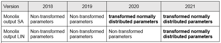
correlationEstimatesSA.txt and/or correlationEstimatesLin.txt
Description: correlation matrix for the (untransformed) parameters
Outputs: matrix with the project parameters as lines and columns. First column contains the parameter names.
The correlation matrix is calculated as:
$$\text{corr}(\theta_i,\theta_j)=\frac{\text{covar}(\theta_i,\theta_j)}{\sqrt{\text{var}(\theta_i)}\sqrt{\text{var}(\theta_j)}}$$
This implies that the diagonal is unitary. The variance-covariance matrix for the untransformed parameters \(\theta\) is obtained from the inverse of the Fisher Information Matrix and the jacobian. See above for the formula.
Log-Likelihood calculation
summary.txt
Description: summary file.
Outputs:
- Header: project file name, date and time of run, Monolix version (outputted population parameter estimation task)
- Estimation of the population parameters: Estimated population parameters & computation time (outputted population parameter estimation task). Standard errors and relative standard errors are added.
- Correlation matrix of the estimates: correlation matrix by block, eigenvalues and computation time
- Log-likelihood Estimation: -2*log-likelihood, AIC and BIC values, together with the computation time
All the more detailed files are in the LogLikelihood folder of the result folder
logLikelihood.txt
Description: Summary of the log-likelihood calculation with the two methods.
Outputs:
- criteria: OFV (Objective Function Value), AIC (Akaike Information Criteria), and BIC (Bayesian Information Criteria )
- method: ImportanceSampling and/or linearization
individualLL.txt
Description: -2LL for each individual. Notice that we only have one by individual even if there are occasions.
Outputs:
- ID: subject name
- method: ImportanceSampling and/or linearization
Tests
Tables
predictions.txt
Description: predictions at the observation times
Outputs:
- ID: subject name. If there are occasions, additional columns will be added to describe the occasions.
- time: Time from the data set.
- MeasurementName: Measurement from the data set.
- RegressorName: Regressor value.
- popPred_medianCOV: prediction using the population parameters and the median covariates.
- popPred: prediction using the population parameters and the covariates, e.g \(V_i=V_{pop}\left(\frac{WT_i}{70}\right)^{\beta}\) (without random effects).
- indivPred_SAEM: prediction using the mean of the conditional distribution, calculated using the last iterations of the SAEM algorithm.
- indPred_mean (if conditional distribution was computed): prediction using the mean of the conditional distribution, calculated in the Conditional distribution task.
- indPred_mode (if conditional mode was computed): prediction using the mode of the conditional distribution, calculated in the EBEs task.
- indWRes_SAEM: weighted residuals \(IWRES_{ij}=\frac{y_{ij}-f(t_{ij}, \psi_i)}{g(t_{ij}, \psi_i)}\) with \(\psi_i\) the mean of the conditional distribution, calculated using the last iterations of the SAEM algorithm.
- indWRes_mean (if conditional distribution was computed): weighted residuals \(IWRES_{ij}=\frac{y_{ij}-f(t_{ij}, \psi_i)}{g(t_{ij}, \psi_i)}\) with \(\psi_i\) the mean of the conditional distribution, calculated in the Conditional distribution task.
- indWRes_mode (if conditional mode was computed): weighted residuals \(IWRES_{ij}=\frac{y_{ij}-f(t_{ij}, \psi_i)}{g(t_{ij}, \psi_i)}\) with \(\psi_i\) the mode of the conditional distribution, calculated in the EBEs task.
Notice that in case of several outputs, Monolix generates predictions1.txt, predictions2.txt, …
Below is a correspondence of the terms used for predictions in Nonmem versus Monolix:
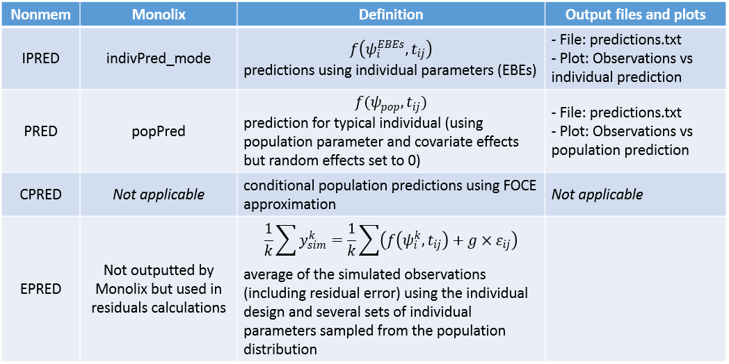
Charts data
All plots generated by Monolix can be exported as a figure or as text files in order to be able to plot it in another way or with other software for more flexibility. The description of all generated text files is described here.
5.6.Reproducibility of MonolixSuite results
Consistent reload of MonolixSuite projects and results
- MonolixSuite applications save in each project all the elements necessary to run the analysis and replicate results from submitted analyses. In practice, the path to the dataset file, the path to the model file (if custom model not from library), and all settings chosen in the Monolix GUI (tagging of the data set columns, initial parameter values, statistical model definition, task settings, seed of the random number generator, etc) are saved in the .mlxtran file. When an existing Monolix project is loaded and re-run, the results will be exactly the same as for the first run.
- In addition, the results of the analysis are loaded in the interface from the results folder as valid results only if nothing has changed in the project since the time of the run. In practice, when launching a run, the content of the mlxtran file is saved in the result folder. When a Monolix project is reloaded, the content of the loaded mlxtran file and the information in the result folder is compared. If they are the same, it means that the results present in the result folder are consistent with the loaded mlxtran and that therefore they are valid. If anything that could affect the results has changed (e.g initial values indicated in the loaded mlxtran file are different from the initial values used to generate the results), the results are not loaded and the warning message “Results have not been loaded due to an old inconsistent project” appears.
- Starting with the 2021R1 version, in Monolix and PKanalix a fingerprint of the dataset is also generated and checked when the project is loaded to ensure that not only the path to the data set file but also the content of the dataset has not been modified.
- Plot settings are saved in a different file (not the .mlxtran file) and do not impact the reloading of the results.
Rerunning a project with the same MonolixSuite version and the same OS (because random number generators are different in Windows, Linux and Mac) yields the exact same results if nothing has changed in the project. The software version used to generate the results is displayed in the file summary.txt in the results folder.
History of runs
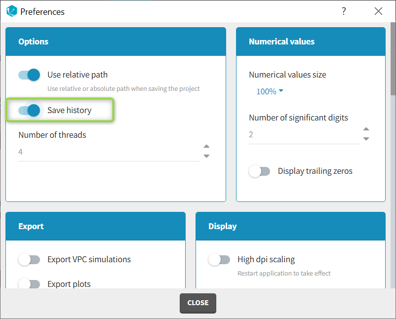
5.7.Comments
Starting from the 2019 version, it is possible to add comments to the project with a dedicated part in the interface in the frame “Comments” as in the following figure.
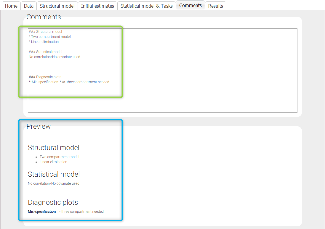 It allows to put information on the project and save it within the project. Notice that you can put information before running the project and/or after running the project and the plots to comment the VPC for example. The text can be formatted with HTML markup or markdown syntax. A preview window is also proposed in order to see the formatted text.
The comments are displayed in Sycomore.
6.Plots
6.1.Overview
6.1.1.Generating and exporting plots
- Generating plots
- List of available plots
- Exporting plots and setting plot-related preferences
- Plots settings
Generating plots
Diagnostic plots can be generated by clickin on the task “Plots” or as part of the scenario when clicking on Run. By default, when reloading a project which has already run, only the plots Observed data and Covariate viewer are displayed. To generate the other diagnostic plots, click on the Plot task. Generating plots automatically at project load can be enabled via a Preference.
The set of plots to compute can be selected by clicking on the button next to the task as shown below, prior to running the task.
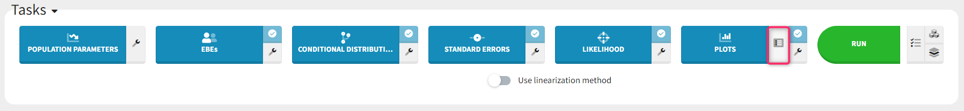
By default, only a subset of plots are selected (see below), with one occurence for each plot. The number of occurences can be selected via the number selection box. Having several occurences of the same plot allows to choose different settings for each occurence, for instance one on linear scale and and one on log scale. The plot selection and number of occurences is saved as part of the mlxtran file upon save, and reapplied at project reload.
The green arrow can be used to generate only one plot type with the given number of occurences without re-generating all other plots. The “+” button allows to add one additional occurence. If the information necessary to generate a plot is not available, these buttons are hidden.
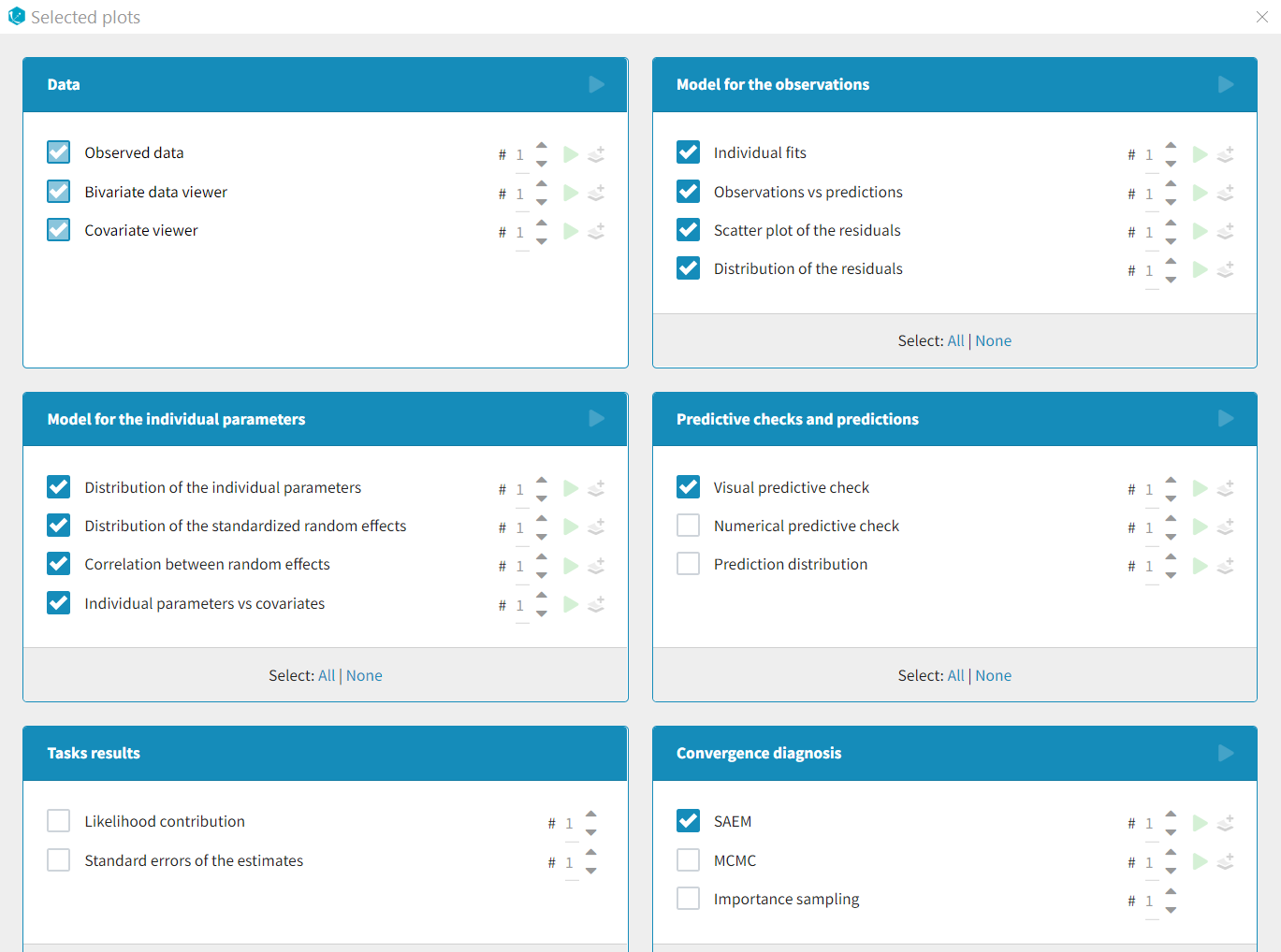
List of available plots
Data
- Observed data: This plot displays the original data w.r.t. time as a spaghetti plot, along with some additional information.
Model for the observations
- Individual fits: This plot displays the individual fits: individual predictions using the individual parameters and the individual covariates w.r.t. time on a continuous grid, with the observed data overlaid.
- Observations vs predictions: This plot displays observations w.r.t. the predictions computed using the population parameters or the individual parameters.
- Scatter plot of the residuals: This plot displays the PWRES (population weighted residuals), the IWRES (individual weighted residuals), and the NPDE (Normalized Prediction Distribution Errors) w.r.t. the time and the prediction.
- Distribution of the residuals: This plot displays the distributions of PWRES, IWRES and NPDE as histograms for the probability density function (PDF) or as cumulative distribution functions (CDF).
Diagnosis plots based on individual parameters
- Distribution of the individual parameters: This plot displays the estimated population distributions overlaid with a histogram of the individual parameters
- Distribution of the random effects: This plot displays the estimated populated distribution of the random effects overlaid with a histogram of the random effects derived from the individual parameters.
- Correlation between random effects: This plot displays scatter plots for each pair of random effects.
- Individual parameters vs covariates: This plot displays the individual parameters or random effects w.r.t. the covariates.
Predictive checks and predictions
- Visual predictive checks: This plot displays the Visual Predictive Check.
- Numerical predictive checks: This plot displays the numerical predictive check.
- BLQ predictive checks: This plot displays the predicted and observed proportion of censored data w.r.t. time.
- Prediction distribution: This plot displays the prediction distribution.
Convergence diagnosis
- SAEM: This plot displays the convergence trajectories of the population parameters estimated with SAEM with respect to the iteration number.
- MCMC: This plot displays the convergence of the Markov Chain Monte Carlo algorithm for the individual parameters estimation.
- Importance sampling: This plot displays the convergence of log-likelihood estimation by importance sampling.
Tasks results
- Likelihood contribution: This plot displays the contribution of each individual to the log-likelihood.
- Standard errors for the estimates: This plot displays the relative standard errors (in %) for the population parameters.
Exporting plots and setting plot-related preferences
Several features can be used to export plots or plot data or create plots automatically:
- Saving a single plot as image (icon button)
- Create plots at project load (Preference)
- Save charts data as binary file (Preference)
- Export VPC simulations (Preference and Export menu)
- Export charts datasets (Preference and Export menu)
- Export plots (Preference and Export menu)
- Export charts data (Preference and Export menu)
Each feature is detailed below in this section.
Most of them are located:
- in the Export menu: to export the plots as image file or a text files for a single project.
- in the Preferences: to export the plots as image file or a text files automatically at the end of each plot generation task. Preferences are user-specific and apply to all projects. The preferences are saved in C:\Users\<username>\lixoft\monolix\monolixXXXXRX\config\config.ini.
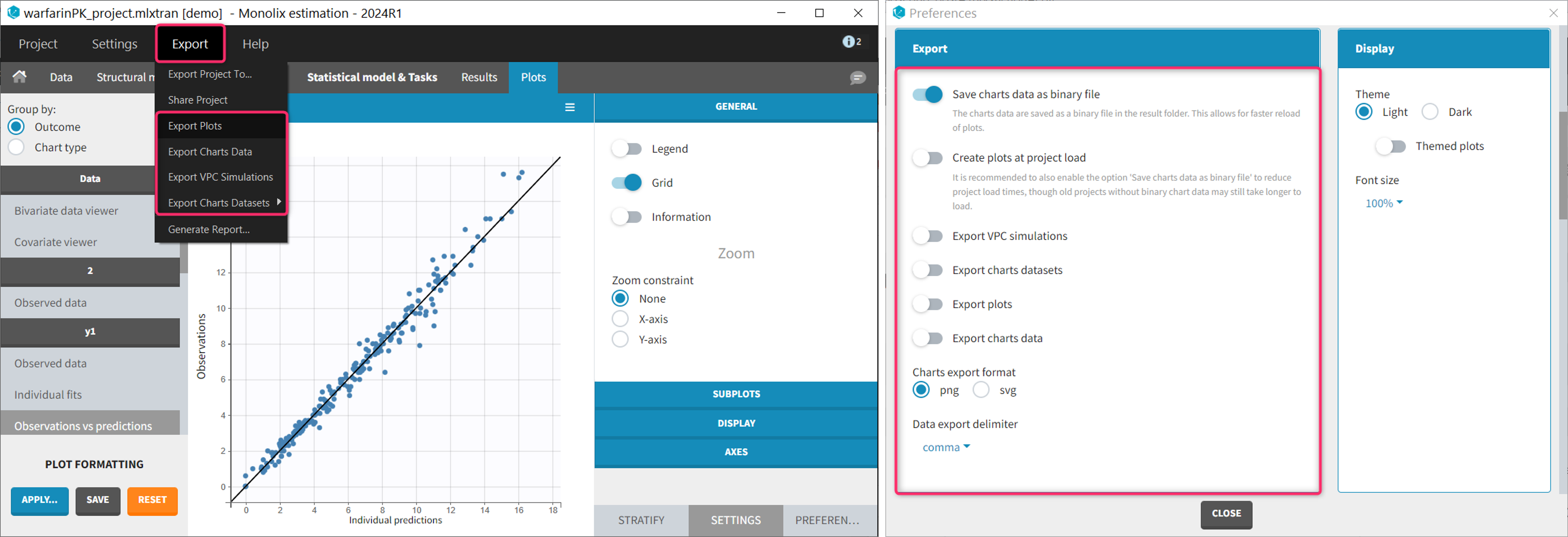
Saving a single plot as image (icon button)
The user can choose to export each plot as an image with an icon on top of the plot, choosing between png and svg format. The files are saved in <result folder>/ChartsFigures with the name of the plot, the observation name (e.g y1 or y2) and a postfix indicating the plot occurence, and page number. Note that information frames are not exported. The icon becomes available only when a structural model has been selected.
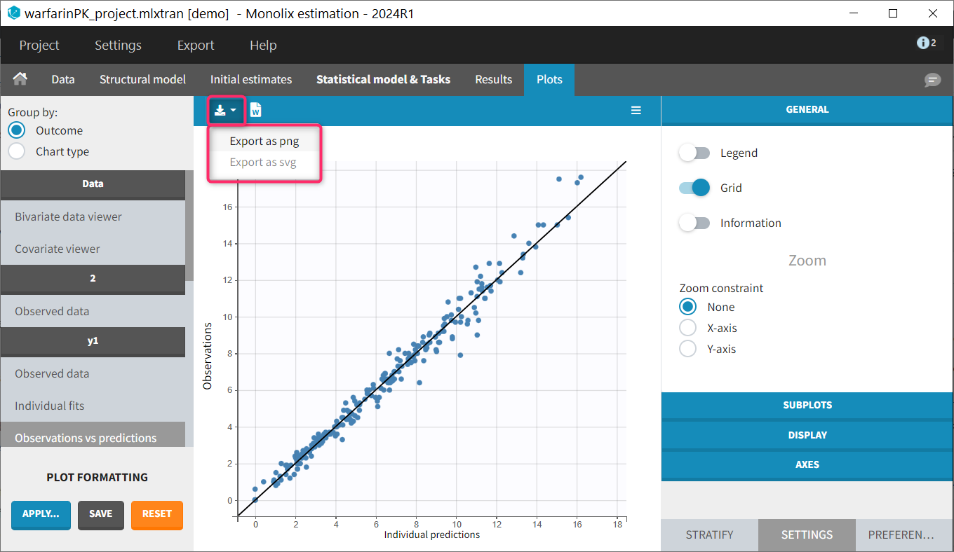
Create plots at project load (Preference)
By default, when a project which has already run is re-opened, only the plots “Observed data” and “Covariate viewer” are displayed. To generate the other diagnostic plots, it is necessary to click on the “Plots” task. Note that it is not necessary to rerun the entire scenario of all tasks.
Starting with version 2024, it is possible to choose whether plots should be created automatically at project load. This option is available in Settings > Preferences > Create plots at project load. When this option is “on”, plots are generated when opening a project with results. Note that this increases the load time, in particular if the charts data have not been saved as binary (see below). By default, the option is “off”.
Save charts data as binary file (Preference)
Generating the plots can take several minutes depending on the model and dataset, because it requires to redo the simulations used in the VPC for instance. Starting with version 2024, it is possible to save the charts data (in particular the simulations) as a binary file, which is re-used when the plots are re-generated. This greatly speeds up the time necessary to generate the diagnostic plots. This option is available in Settings > Preferences > Save charts data as binary file. When this option is “on” (default), the charts data are saved in a non-human-readable format in <result folder>/ChartsData/.Internals/chartsData.dat each time the plots are generated. At project reload, if the file chartsData.dat exists and is valid, it is used to generate the plots faster.
Export VPC simulations (Preference and Export menu)
Simulations used to generate the VPC plot can be exported as txt file. This allows to replot the VPC with an external software for instance. If this export is required for a single project, the user can click Export > Export VPC simulations. The simulations are saved in <result folder>\ChartsData\VisualPredictiveCheck\XXX_simulations.txt. If the user wishes to do this export each time the VPC plot is generated, the option Settings > Preferences > Export VPC simulations can be set to “on”.
Export charts datasets (Preference and Export menu)
Simulations used for the VPC and the Individual fits (prediction on a fine time grid) can be exported as MonolixSuite-formatted datasets (including dose records, regressors, etc). This is useful if these simulations need to be loaded in another MonolixSuite application such as PKanalix for instance. To export these formatted simulations once use Export > Export Charts Datasets > VPC or Individual fits. A pop-up window will let you choose the name and location of the saved files.
To export the simulations as formatted dataset systematically each time the plots are generated, the option Settings > Preferences > Export charts datasets can be set to “on”. The files are saved in <result folder>/DataFile/ChartsData/indfits_data.csv and vpc_data.csv.
Export plots (Preference and Export menu)
Plots can be saved as image files. To save a single plot, use the icon on the top of the plot (see section above). To save all plots for a single project, use Export > Export plots. To systematically save all generated plots as image file, set the the option Settings > Preferences > Explot plots to “on”. The files are saved in <result folder>/ChartsFigures with the name of the plot, the observation name (e.g y1 or y2) and a postfix indicating the plot occurence, and page number. The files are saved at the end of the plot generation task. The file format (png or svg) can be chosen in the Preferences. Note that information frames are not exported.
Export charts data (Preference and Export menu)
The values used to draw the plots can be saved as txt files. This can be useful to regenerate the plots using an external tool. To export the charts data for a single project, use Export > Export charts data. To systematically export the charts data at the end of the plot generation, set the the option Settings > Preferences > Explot charts data to “on”. The files are saved in <result folder>/ChartsData with one subfolder per plot. The content of each file is described on the dedicated page. The file separator can be chosen in the Preferences.
Plot settings
A few plot settings impact the simulations required for the plots. They can be chosen in the Settings panel for the Plots task.
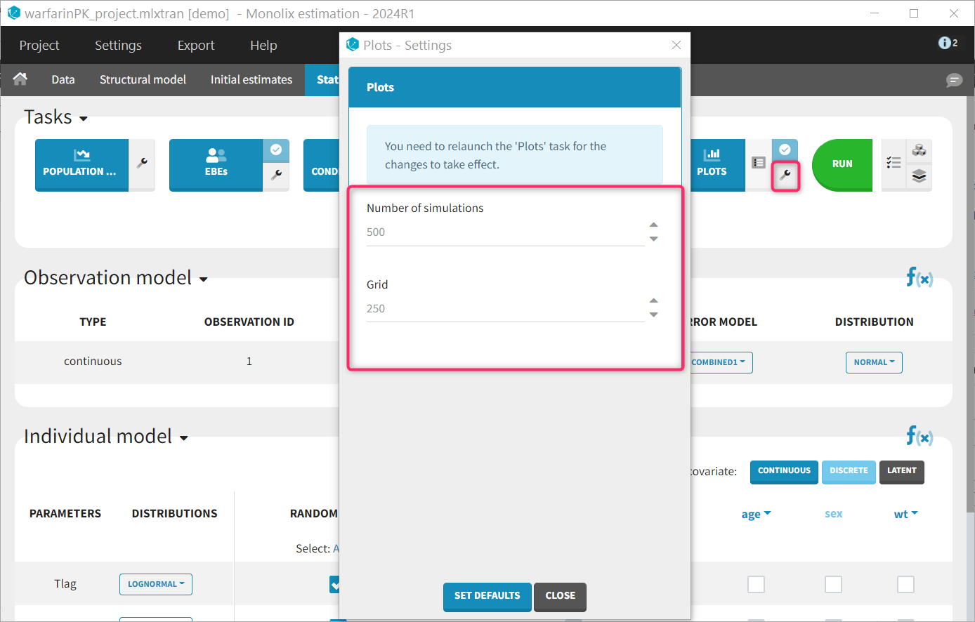
- Number of simulations: number of replicates simulated for the VPC, NPC and Prediction distribution plot (default: 500)
- Grid: number of points of the fine time grid used for the individuals fits (default: 250). See the video below for more details.
6.1.2.Interacting with the plots
- Interacting with the plots
- Highlight: tooltips and ID
- Stratification: split, color, filter
- Layout
- Preferences: customizing the plot appearance
Interactive diagnostic plots
In the PLOTS tab, the right panel has several sub – tabs (at the bottom) to interact with the plots:
- The tab “Settings” provides options specific to each plot, such as hiding or displaying elements of the plot, modifying some elements, or changing axes scales, ticks and limits.
- The tab “Stratify” can be used to select one or several covariates for splitting, filtering or coloring the points of the plot. See below for more details.
- The tab “Preferences” alows to customize graphical aspects such as colors, font size, dot radius, line width, …
These tabs are marked in purple on the following figure, which is the panel that is showed for observed data:
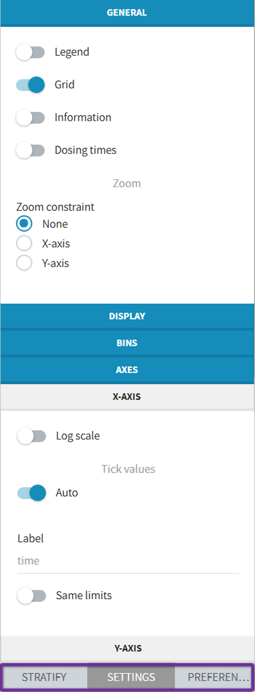
Highlight: tooltips and ID
In all the plots, when you hover a point or a curve with your mouse, some informations are provided as tooltips. For example, the ID is displayed when hovering a point or the curve of an individual in the observed data plot, the ID, the time and/or the prediction is displayed in the scatter plot of the residuals.
In addition, starting from the 2019 version, when hovering one point/ID in a plot, the same ID will be highlighted in all the plots with the same color.
Stratification: split, color, filter
The stratification panel allows to create and use covariates for stratification purposes. It is possible to select one or several covariates for splitting, filtering or coloring the data set or the diagnosis plots as exposed on the following video.
The following figure shows a plot of the observed data from the warfarin dataset, stratified by coloring individuals according to the continuous covariate wt: the observed data is divided into three groups, which were set to equal size with the button “rescale”. It is also possible to set groups of equal width, or to personalize dividing values.
In addition, the bounds of the continuous covariate groups can be changed manually.
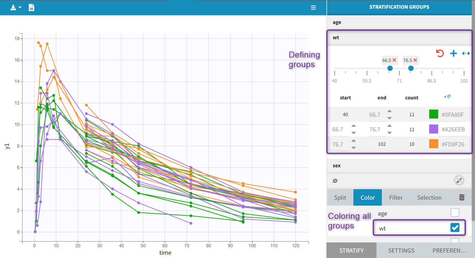 Moreover, clicking on a group highlights only the individuals belonging to this group, as can be seen below:
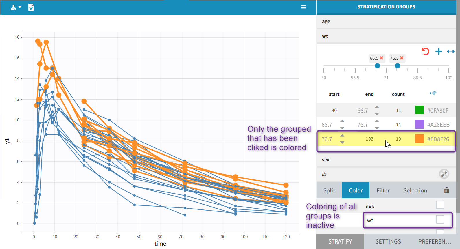
Values of categorical covariates can also be assigned to new groups, which can then be used for stratification.
In addition, the number of subjects in each categorical covariate groups is displayed.
Starting from the 2021R1 version, the list of subplots obtained by split is displayed below the split selection. It is possible to reorder the items in this list with drag-and-drop, which also reorders the subplot layout. Moreover, an “edit” icon next to each subplot name in the list allows to change the subplot titles.
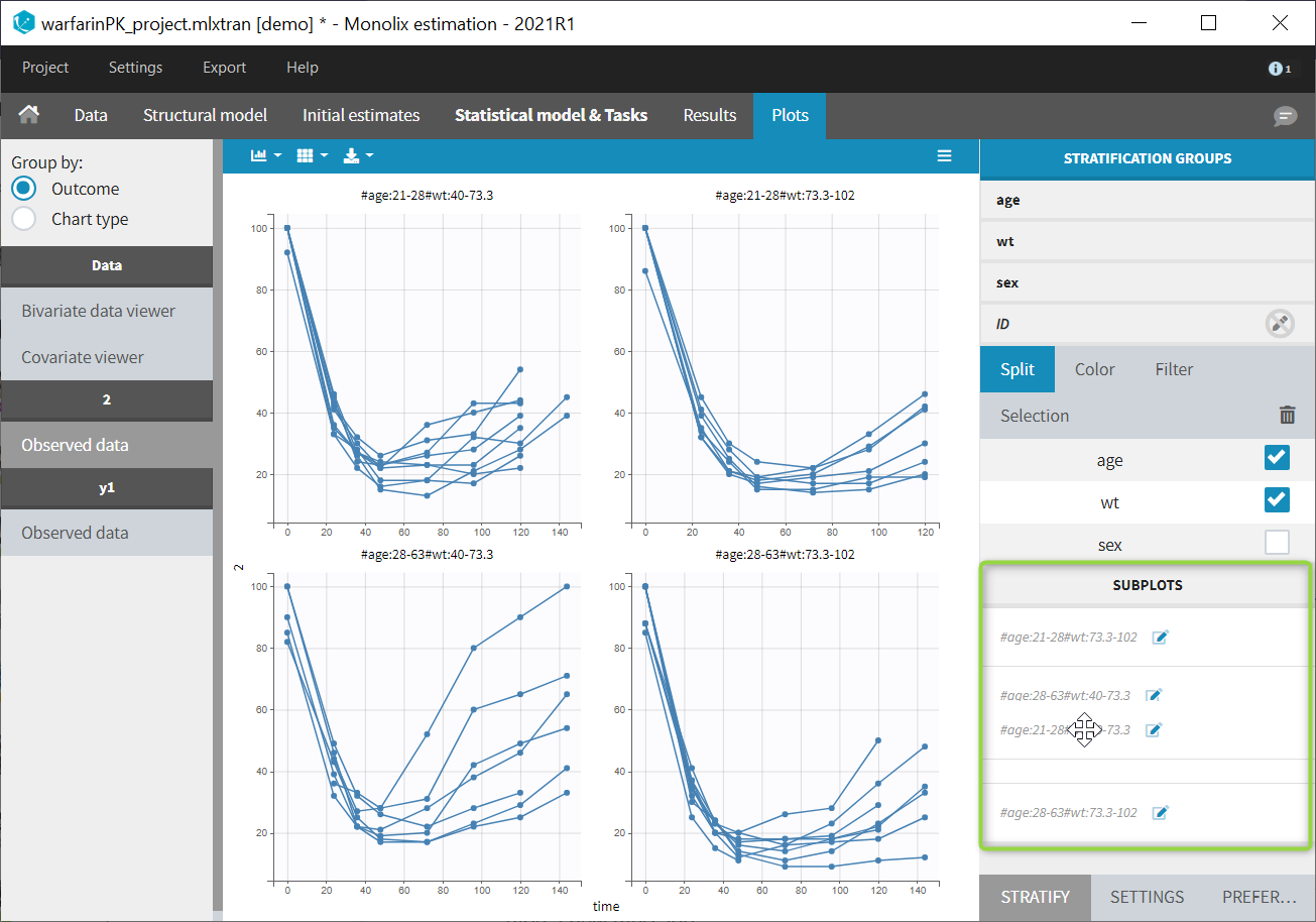
Preferences: customizing the plot appearance
In the “preferences” tab, the user can modify the different aspects of the plot: colors, line style and width, fonts and label position offsets, …
The following figures show on the warfarin demo the choices for the plot content and the choices for the labels and titles (in the “Plotting region” section). The sizes of all elements of the plots can also be changed with the single “zoom” preference in “Plotting region”.
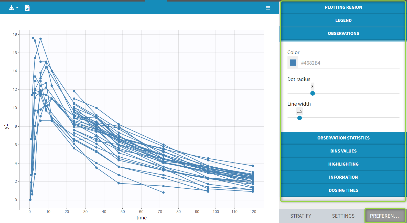
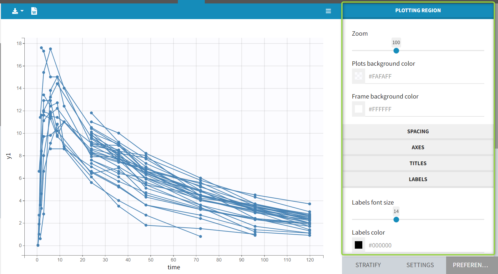
Layout
The layout can be modified with buttons on top of each plot.
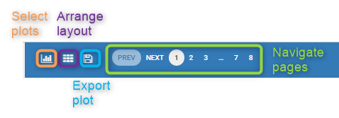
The first button can be used to select a set of subplots to display in the page. For example, as shown below, it is possible to display 9 individual fits per page instead of 12 (default number). The layout is then automatically adapted to balance the number of rows and columns.
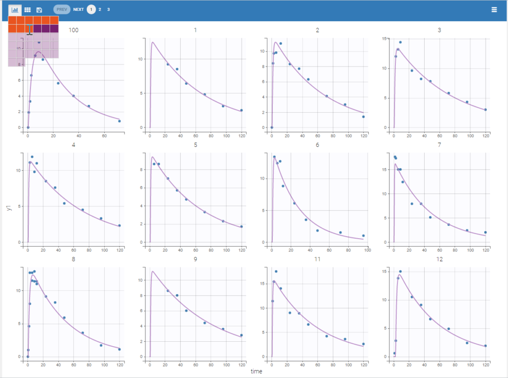
The second button can be used to choose a custom layout (number of rows and columns). On the example figures below, the default layout with 3 subplots (left) is modified to arrange them on a single column (right).
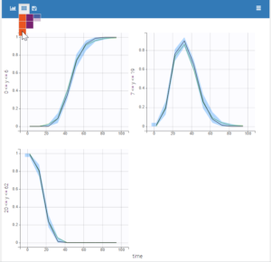
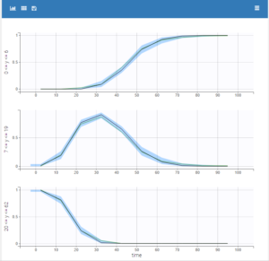
6.1.3.Transferring plot formatting
Note: the features described on this page are not available in MonolixSuite versions prior to 2024R1.
MonolixSuite offers the ability to transfer plot formatting from one plot to another within the same project or across projects. This can save you time and effort when you want to apply the same formatting options, such as stratification, preferences, or settings, to multiple plots, or when you want to use the same plot formatting for different analyses or datasets.
- Transferring plot formatting within one project
- Transferring plot formatting across projects with plot presets
- Applying pre-defined plot formatting
- Restoring default plot formatting
Transferring plot formatting within one project
To transfer plot formatting within one project, you need to use the “Apply…” button on the bottom left of the Plots tab and select “From plot” in the window that opens:


Selecting the source and target plots
The window allows you to select the source plot, which is the plot that has the formatting you want to transfer, and the target plots, which are the plots that you want to apply the formatting to. You can select all plots by clicking on the Select all button, or select all plots specific to some observation id with the “Fast selection”, or corresponding to an occurrence rank if some plots have been generated with several occurences.
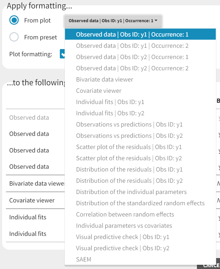
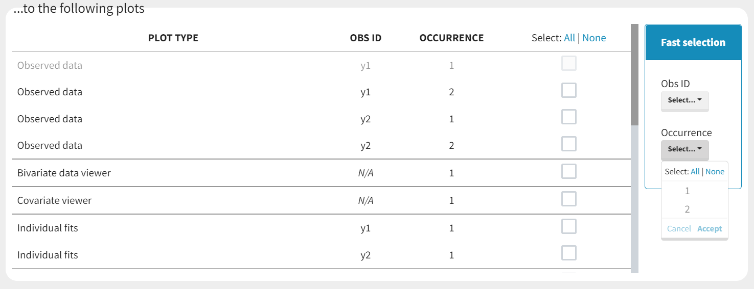
Choosing the sections to transfer
You can also choose which sections of the configuration you want to transfer: Stratify, Settings, or Preferences.
![]()
By default, Stratify and Preferences are selected.
- The Stratify section includes the options to stratify the plots by covariates or occasions.
- The Settings section includes the options to customize the content of the plots: elements displayed or not on the plots, such as the legend, the grid, the observed data points, etc, and calculation settings such as the axes, bins etc.
- The Preferences section includes the options to change the colors, fonts, sizes, etc.
Once you have selected the source plot, the target plots, and the sections to transfer, you can click on the Apply button to transfer the plot configurations.
Transferring plot formatting across projects with plot presets
To transfer plot formatting across different projects, you need to use the plot presets feature, which allows you to define and apply presets for plot configurations.
Defining a plot preset
To define a plot preset, you need to first set up your plot configuration as you would like by choosing the stratification, preferences, and settings options for each plot (you can use the transfer or plot formatting between plots within the same project, described in the first section, to help you). Then, you can save this configuration as a preset by clicking on the Save icon in the Apply from the Plot Formatting panel:

You will be asked to give a name and a description to your preset, and to select which sections of the formatting you want to include in the preset among Stratify, Settings and Preferences. If the project has several types of observations, only the plots corresponding to one of them can be used to define the preset so it is necessary to select the observation id. You can also choose to set this preset as your default, which means that when creating a new project or when you click on Reset, the plot formatting from this preset will be applied instead of the system default.
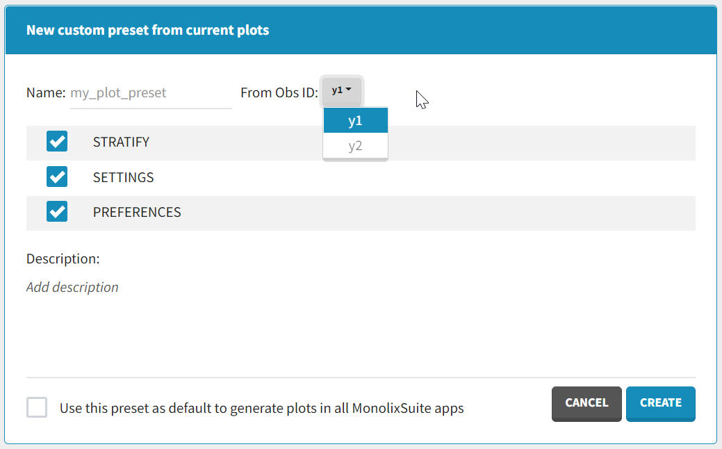
Applying a plot preset
After saving your preset, it will be available in the list of presets that you can choose from when you click on “From preset” in the window that opens with “Apply…” in the Plot Formatting panel.
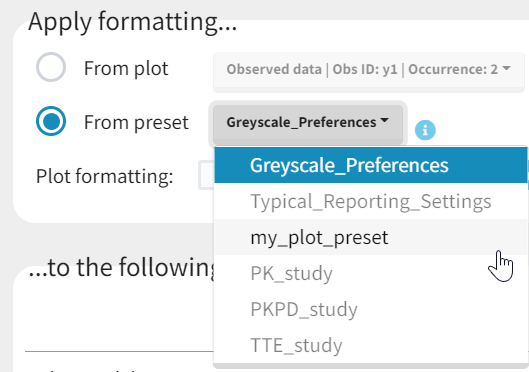
You can apply your preset to a list of plots in another project, by opening this project, clicking on “Apply…” and “From preset” and by selecting the preset and the target plots, and finally clicking on Apply. This will transfer the plot configurations from the preset to the target plots.
The target plots must be:
- the same type of plots that were used to define the preset: for example if no VPC had been generated in the project used to define the preset, then the plot preset cannot be applied to a VPC in a new project, as there is no VPC formatting option to apply. The VPC will be greyed out in the list of target plots.
- the same plot occurrence that was used to define the preset: for example if the project used to define the preset had only one VPC occurrence, and you want to apply that preset in a project where you have generated two VPC occurrences, then the second VPC occurrence will be greyed out in the list of target plots.
Note that axis limits values and bins settings are not saved as part of the preset because they are considered too project-specific.
Please note this major difference between “Apply formatting from plot” and “Apply formatting from preset”:
- “Apply formatting from plot” applies all selected options from the source plot to all selected target plots. Thus, if you select a VPC stratified by STUDY as source plot and the Observed data plot as target plot, and “Stratify” section in plot formatting to be transfer, you will obtain the Observed data plot stratified by STUDY.
- “Apply formatting from preset” applies the selected options from each plot saved in the preset to the corresponding plot in your project. Thus, if you saved a preset including the “Stratify” section based on a project where the VPC is stratified by STUDY but not the Observed data plot, applying that preset to another project will stratify the VPC by STUDY but not the Observed data plot.
Managing plot presets
You can also manage your presets by going to Settings > Manage presets > Plot formatting.
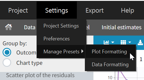
This will open a window where you can see all presets, modify, update or remove your custom presets, and export or import them as separate files with a lixpst extension. That way you can easily share your presets with your colleagues or collaborators to standardize your plot formatting.
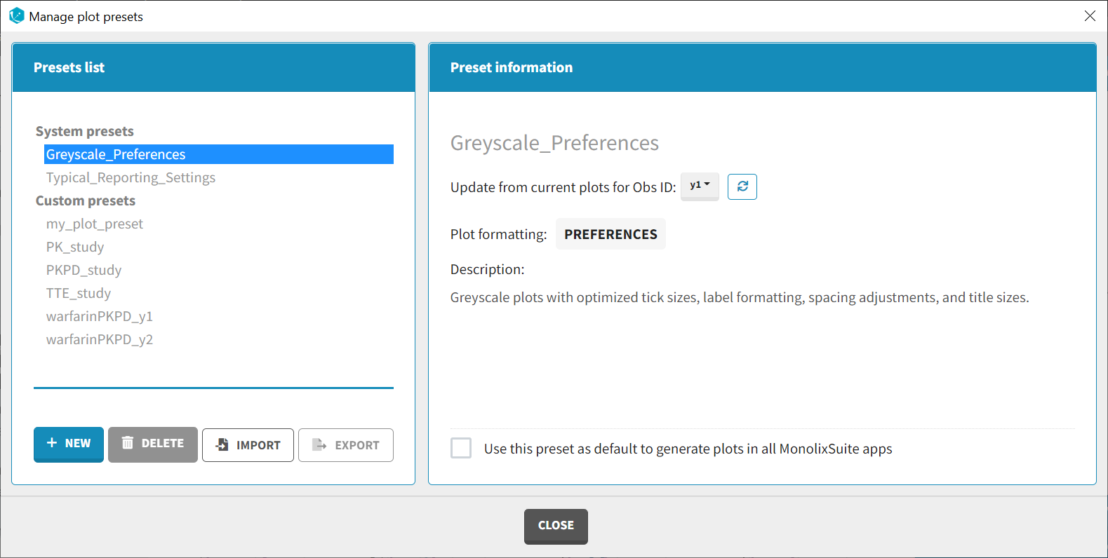
Applying pre-defined plot formatting
In addition to your custom presets, MonolixSuite also provides two pre-defined presets that you can use to apply plot formatting. These presets are:
- Greyscale_Preferences: This preset affects only the Preferences section of the plot configurations, and produces publication-ready greyscale plots with optimized size and spacing of the texts to improve readability of the plots (example shown below for the VPC).

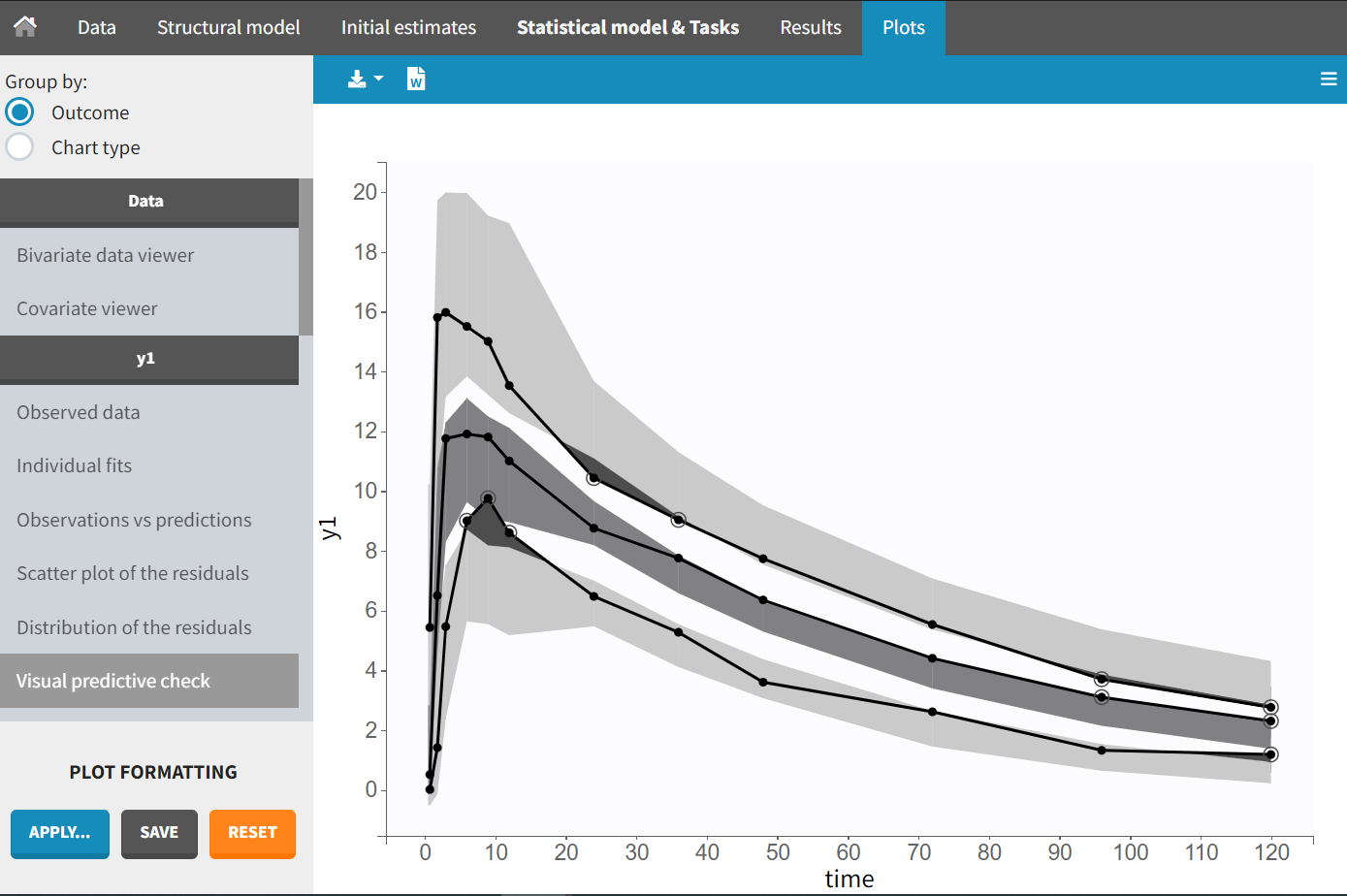
- Typical_Reporting_Settings: This preset affects only the Settings section of the plot configuration, and corresponds to plot settings typically chosen to report the analysis results. In addition to removing the grid in the background for all plots:
- VPC: observed data points and predicted percentiles are displayed (see example below)
- Observation vs Predictions: Observations vs Population Predictions are displayed in addition to Observations vs Individual Predictions
- Scatterplot of the residuals: Population residuals and NPDE are displayed in addition to Individual residuals.


You can apply these presets to any plot in your project by selecting them from the list of presets and clicking on Apply. You can also combine these presets with your own presets or with the Apply from plot feature, to create the plot configuration that suits your needs.
Restoring default plot configuration
Using the Reset button
If you want to restore the default plot configuration, you can click on the Reset icon in the Apply from plot panel. This will reset all plots to the system default, or to your custom default if you have defined one.

Note that resetting the plot configuration will not affect the plot presets that you have defined or imported. You can still apply them to any plot after resetting.
Defining a custom default
To define a custom default, you need to create a preset and select the option “Use this preset as default” when saving it. This will make this preset the default configuration for all plots. You can also unset a preset as default by going to Settings > Manage presets > Plot formatting, and unchecking the option “Use this preset as default” for the preset.
6.1.4.Export charts
All plots generated by Monolix can be exported
All plots generated by Monolix can be exported as a figure or as text files in order to be able to plot it in another way or with other software for more flexibility.
All the files can be exported in R for example using the following command
read.table("/path/to/file.txt", sep = ",", comment.char = "", header = T)
Remarks
- The separator is the one defined in the user preferences. We set “,” in this example as it is the one by default.
- The command comment.char = "" is needed for some files because to define groups or color, we use the character # that can be interpreted as a comment character by R.
The list of plots below corresponds to all the plots that Monolix can generate. They are computed with the task “Plots”, and the list of plots to compute can be selected by clicking on the button next to the task as shown below, prior to running the task.
Exporting the charts data can be made through the Export menu or through the preferences as described here.
In the following, we describe all the files generated by the export function
- Charts concerning the Data (Observed data).
- Charts concerning the model for the observations (Individual fits, Observations vs predictions, Scatter plot of the residuals, Distribution of the residuals
- Charts concerning the model for the individual parameters (Distribution of the individual parameters, Distribution of the random effects, Correlation between random effects, Individual parameters vs covariates)
- Charts concerning the predictive checks and predictions (Visual predictive checks, Numerical predictive checks, BLQ predictive checks, Prediction distribution)
- Charts concerning the convergence diagnosis (SAEM, MCMC) and the tasks results (Standard errors for the estimates)
Charts concerning the Data
Observed data (continuous, categorical, and count)
xxx_observations.txt
Description: observation values
Full output file description
| Column | Description | Comment |
| id | Subject identifier | – |
| OCC | Occasion value | (optional) if there is IOV in the data set |
| time | Observation time | – |
| y | Observation value (loq) | The name of the column is the observation name |
| censored | 1 if the observation is censored, 0 otherwise | – |
| split | Name of the split the subject belongs to | – |
| color | Name of the color the observation is colored with | – |
| filter | 1 if the subject is filtered, 0 otherwise | – |
Observed data (event)
xxx_curves.txt
Description: observation values
Full output file description
| Column | Description | Needed Task |
| time | Observation times | – |
| survivalFunction | Survival of first event | – |
| averageEventNumber | Average number of event at that time | – |
| split | Name of the split the subject occasion belongs to | – |
xxx_censored.txt
Description: censored values
Full output file description
| Column | Description | Needed Task |
| time | Observation times | – |
| values | Survival of first event | – |
| split | Name of the split the subject occasion belongs to | – |
Model for the observations
Individual Fits
xxx_observations.txt
Description: observation values
Full output file description
| Column | Description | Comment |
| id | Subject identifier | – |
| OCC | Occasion value | (optional) if there is IOV in the data set |
| time | Observation time | – |
| y | Observation value (loq) | – |
| median | Prediction interval median | – |
| piLower | Lower percentile of the individual prediction interval | – |
| piUpper | Upper percentile of the individual prediction interval | – |
| censored | 1 if the observation is censored, 0 otherwise | – |
xxx_fits.txt
Description: individual fits based on population parameters and individual parameters
Full output file description
| Column | Description | Needed Task |
| id | Subject identifier | – |
| OCC | Occasion value | (optional) if there is IOV in the data set |
| time | Continuous time grid used to compute fits | – |
| pop | Prediction using population parameter values and average covariate value from the population (continuous) or reference covariate value (categorical). | – |
| popPred | Prediction using population parameter values and individual covariates. | – |
| indivPredMean | Prediction based on the individual parameter values estimated by conditional mean | Conditional distribution need to be computed |
| indivPredMode | Prediction based on the individual parameter values estimated by conditional mode | EBEs need to be computed |
Observation vs Prediction
xxx_obsVsPred.txt
Description: observation and prediction (pop & indiv) values
Full output file description
| Column | Description | Needed Task |
| id | Subject identifier | – |
| OCC | Occasion value | (optional) if there is IOV in the data set |
| time | time of the observation | |
| y | Observation value (loq) | – |
| y_simBlq | Observation value (simulated blq) | |
| popPred | Predictions based on population parameter values | |
| indivPredMean | Predictions based on the individual parameter values estimated by conditional mean | Conditional distribution need to be computed |
| indivPredMode | Predictions based on the individual parameter values estimated by conditional mode | EBEs need to be computed |
| censored | 1 if the observation is censored, 0 otherwise | |
| split | Name of the split the subject occasion belongs to | |
| color | Name of the color the observation is colored with | |
| filter | 1 if the subject is filtered, 0 otherwise | – |
xxx_obsVsSimulatedPred.txt
Description: observation and simulated prediction values
Full output file description
| Column | Description | Needed Task |
| rep | Replicate id | |
| id | Subject identifier | – |
| OCC | Occasion value | (optional) if there is IOV in the data set |
| time | time of the observation | |
| y | Observation value (loq) | – |
| y_simBlq | Observation value (simulated blq) | |
| indivPredSimulated | Predictions based on the simulated individual parameter values estimated by conditional distribution | Conditional distribution need to be computed |
| censored | 1 if the observation is censored, 0 otherwise | |
| split | Name of the split the subject occasion belongs to | |
| color | Name of the color the observation is colored with | |
| filter | 1 if the subject is filtered, 0 otherwise |
xxx_visualGuides.txt
Description: splines and confidence intervals for predictions
Full output file description
| Column | Description | Needed Task |
| popPred | Continuous grid over population prediction values | – |
| popPred_spline | Spline ordinates for population predictions | – |
| popPred_piLower | Lower percentile of prediction interval for population predictions | – |
| popPred_piUpper | Upper percentile of prediction interval for population predictions | – |
| indivPred | Continuous grid over individual prediction values | – |
| indivPred_spline | Spline ordinates for individual predictions | – |
| indivPred_piLower | Lower percentile of prediction interval for individual predictions | – |
| indivPred_piUpper | Upper percentile of prediction interval for individual predictions | – |
| split | Name of the split the visual guides belong to |
Distribution of the residuals
xxx_pdf.txt
Description: probability density function of each residual type (pwres, iwres, npde)
Full output file description
| Column | Description | Needed Task |
| pwRes_abscissa | Abscissa for pwres pdf | – |
| pwRes_pdf | Pdf of pwres | – |
| iwRes_abscissa | Abscissa for iwres pdf | – |
| iwRes_pdf | Pdf of the iwres | – |
| npde_abscissa | Abscissa for npde pdf | – |
| npde_pdf | Pdf of the npde | – |
| split | – |
xxx_cdf.txt
Description: cumulative distribution function of each residual type (pwres, iwres, npde)
Full output file description
| Column | Description | Needed Task |
| pwRes_abscissa | Abscissa for pwres cdf | – |
| pwRes_cdf | Cdf of pwres | – |
| iwRes_abscissa | Abscissa for iwres cdf | – |
| iwRes_cdf | Cdf of the iwres | – |
| npde_abscissa | Abscissa for npde cdf | – |
| npde_cdf | Cdf of the npde | – |
| split | – |
theoreticalGuides.txt
Description: theoretical guides for the pdf and the cdf
Full output file description
| Column | Description | Needed Task |
| abscissa,pdf,cdf | Abscissa for the theoretical curves | – |
| Theoretical value of the pdf | – | |
| cdf | Theoretical value of the cdf | – |
Scatter plot of the residuals
xxx_prediction_percentiles_iwRes.txt
Description: prediction percentiles of the iwREs to plot iwRes w.r.t. the prediction. The same files exists with the pwres and the npde.
Full output file description
| Column | Description | Needed Task |
| prediction | Value of the prediction | – |
| empirical_median | Empirical median of the iwRes | – |
| empirical_lower | Empirical lower percentile of the iwRes | |
| empirical_upper | Empirical upper percentile of the iwRes | |
| theoretical_median | Theoretical median of the iwRes | |
| theoretical_lower | Theoretical lower of the iwRes | |
| theoretical_upper | Theoretical upper of the iwRes | |
| theoretical_median_piLower | Lower bound of the theoretical median prediction interval | |
| theoretical_median_piUpper | Upper bound of the theoretical median prediction interval | |
| theoretical_lower_piLower | Lower bound of the theoretical lower prediction interval | |
| theoretical_lower_piUpper | Upper bound of the theoretical lower prediction interval | |
| theoretical_upper_piLower | Lower bound of the theoretical upper prediction interval | |
| theoretical_upper_piUpper | Upper bound of the theoretical upper prediction interval | |
| split | Name of the split the subject occasion belongs to |
xxx_time_percentiles_iwRes.txt
Description: time percentiles of the iwREs to plot iwRes w.r.t. the time. The same files exists with the pwres and the npde.
Full output file description
| Column | Description | Needed Task |
| time | Value of the time | – |
| empirical_median | Empirical median of the iwRes | – |
| empirical_lower | Empirical lower percentile of the iwRes | |
| empirical_upper | Empirical upper percentile of the iwRes | |
| theoretical_median | Theoretical median of the iwRes | |
| theoretical_lower | Theoretical lower of the iwRes | |
| theoretical_upper | Theoretical upper of the iwRes | |
| theoretical_median_piLower | Lower bound of the theoretical median prediction interval | |
| theoretical_median_piUpper | Upper bound of the theoretical median prediction interval | |
| theoretical_lower_piLower | Lower bound of the theoretical lower prediction interval | |
| theoretical_lower_piUpper | Upper bound of the theoretical lower prediction interval | |
| theoretical_upper_piLower | Lower bound of the theoretical upper prediction interval | |
| theoretical_upper_piUpper | Upper bound of the theoretical upper prediction interval | |
| split | Name of the split the subject occasion belongs to |
xxx_residuals.txt
Description: residuals values (pwres, iwres, npde)
Full output file description
| Column | Description | Needed Task |
| id | Subject identifier | – |
| OCC | Occasion value | (optional) if there is IOV in the data set |
| time | Observation times | – |
| prediction_pwRes | Predictions based on population parameter values | SAEM |
| pwRes | PwRes (computed with observations) | SAEM |
| pwRes_blq | PwRes (computed with simulated blq) | |
| prediction_iwRes_mean | Predictions based on the individual parameter values estimated by conditional mean (INDIVESTIM) if available, SAEM either | |
| iwRes_mean | IwRes (computed with observations and individual parameter values estimated by conditional mean (INDIVESTIM) if available, SAEM either) | |
| iwRes_mean_simBlq | IwRes (computed with simulated blq and individual parameter values estimated by conditional mean (INDIVESTIM) if available, SAEM either) | |
| prediction_iwRes_mode | Predictions based on the individual parameter values estimated by conditional mode (INDIVESTIM) | |
| iwRes_mode | IwRes (computed with observations and the individual parameter values estimated by conditional mode (INDIVESTIM)) | |
| iwRes_mean_simBlq | IwRes (computed with simulated blq and the individual parameter values estimated by conditional mode (INDIVESTIM)) | |
| prediction_npde | Predictions based on population parameter values | |
| npde | Npde (computed with observations) | |
| npde_simBlq | Npde (computed with simulated blq) | SAEM – If there are some censored data in the data set |
| censored | 1 if the observation is censored, 0 otherwise | |
| split | Name of the split the subject occasion belongs to | |
| color | Name of the color the observation is colored with | |
| filter | 1 if the subject is filtered, 0 otherwise | – |
xxx_simulatedResiduals.txt
Description: simulated residuals values
Full output file description
| Column | Description | Needed Task |
| rep | replicate | – |
| id | Subject identifier | – |
| OCC | Occasion value | (optional) if there is IOV in the data set |
| time | Observation times | – |
| prediction_iwRes | Predictions based on the simulated individual parameter values based on the conditional distribution | |
| iwRes_simulated | IwRes (computed with observations and the simulated individual parameter values) | |
| iwRes_simulated_simBlq | IwRes (computed with simulated blq and the simulated individual parameter values) | |
| censored | 1 if the observation is censored, 0 otherwise | – |
| split | Name of the split the subject occasion belongs to | |
| color | Name of the color the observation is colored with | |
| filter | 1 if the subject is filtered, 0 otherwise | – |
xxx_spline.txt
Description: splines (residuals values against time and prediction)
Full output file description
| Column | Description | Needed Task |
| time_pwRes | Time grid for pwRes spline | SAEM |
| time_pwRes_spline | pwRes against time spline | SAEM |
| time_iwRes | Time grid for iwRes spline | At least SAEM |
| time_iwRes_spline | iwRes against time spline | At least SAEM |
| time_npde | Time grid for npde spline | SAEM |
| time_npde_spline | npde against time spline | SAEM |
| prediction_pwRes | Prediction grid for pwRes spline | SAEM |
| prediction_pwRes_spline | pwRes against population prediction spline | SAEM |
| prediction_iwRes | Prediction grid for iwRes spline | At least SAEM |
| prediction_iwRes_spline | iwRes against individual prediction spline | At least SAEM |
| prediction_npde | Prediction grid for npde spline | SAEM |
| prediction_npde_npde | npde against population prediction spline | SAEM |
| split | Name of the split the visual guides belong to | If the chart is splitted |
xxx_{time,population,individual}Bins.txt
Description: bins values for the corresponding axis.
Full output file description
| Column | Description | Needed Task |
| binsValues | Abscissa bins values | – |
| split | Name of the split the bins refer to | If the chart is splitted |
Model for the individual parameters
Distribution of the individual parameters
cdf.txt
Full output file description
| Column | Description | Needed Task |
| param_abscissa | Abscissa of the cdf of the individual parameter param | – |
| param_cdf | Empirical cdf of the individual parameter param | – |
| split | Name of the split the subject occasion belongs to |
pdf.txt
Full output file description
| Column | Description | Needed Task |
| param_abscissa | Abscissa of the pdf of the individual parameter param | – |
| param_pdf | Empirical pdf of the individual parameter param | – |
| split | Name of the split the subject occasion belongs to |
visualGuides.txt
Full output file description
| Column | Description | Needed Task |
| param_abscissa | Abscissa of the pdf and the pdf of the individual parameter param | – |
| param_pdf | Theoretical pdf of the individual parameter param | – |
| param_cdf | Theoretical cdf of the individual parameter param |
Distribution of the random effects
cdf.txt
Full output file description
| Column | Description | Needed Task |
| param_abscissa | Abscissa of the cdf of the standardized random effect of param | – |
| param_cdf | Empirical cdf of the standardized random effect of param | – |
| split | Name of the split the subject occasion belongs to |
pdf.txt
Full output file description
| Column | Description | Needed Task |
| param_abscissa | Abscissa of the pdf of the standardized random effect of param | – |
| param_pdf | Empirical pdf of the standardized random effect of param | – |
| split | Name of the split the subject occasion belongs to |
StandardizedEta.txt
Description: standardized random effects of the individual parameters
Full output file description
| Column | Description | Needed Task |
| id | Subject identifier | – |
| OCC | Occasion value | (optional) if there is IOV in the data set |
| standEta_X_method | Standardized random effects values on each individual parameter with variability.
It can be StandEta_SAEM, StandEta_Mean, StandEta_Mode |
– |
| filter | 1 if the subject is filtered, 0 otherwise | – |
SimulatedStandardizedEta.txt
Description: simulated standardized random effects of the individual parameters
Full output file description
| Column | Description | Needed Task |
| rep | Replicate id | – |
| id | Subject identifier | – |
| OCC | Occasion value | (optional) if there is IOV in the data set |
| standEta_X_simulated | Standardized random effects values on each individual parameter with variability. | – |
| filter | 1 if the subject is filtered, 0 otherwise | – |
Correlation between Random Effects
eta.txt
Description: standard error on individual parameter predictions
Full output file description
| Column | Description | Needed Task |
| id | Subject identifier | – |
| OCC | Occasion value | (optional) if there is IOV in the data set |
| eta_X_method | Random effects values on each individual parameter with variability. It can be
eta_SAEM, eta_Mean, or eta_Mode |
– |
| color | Name of the color the ID is colored with | – |
| filter | 1 if the subject is filtered, 0 otherwise | – |
simulatedEta.txt
Description: standard error on individual parameter predictions
Full output file description
| Column | Description | Needed Task |
| rep | Replicate number | |
| id | Subject identifier | – |
| OCC | Occasion value | (optional) if there is IOV in the data set |
| eta_X_simulated | Simulated random effects values on each individual parameter | – |
| color | Name of the color the ID is colored with | – |
| filter | 1 if the subject is filtered, 0 otherwise | – |
visualGuides.txt
Description: spline and linear regression for each couple of individual parameters plotted one against the other
This is done for each combination of parameter p1 and p2 to have p1 w.r.t. p2
Full output file description
| Column | Description | Needed Task |
| p1_vs_p2_abscissa | Abscissa | – |
| p1_vs_p2_spline | Spline ordinates | – |
| p1_vs_p2_regression | Linear regression ordinates | – |
Individual Parameters Vs Covariates
covariates.txt
Description: individual parameters and random effects and covariate value for each subject
Full output file description
| Column | Description | Needed Task |
| id | Subject identifier | – |
| OCC | Occasion value | (optional) if there is IOV in the data set |
| trans_X_method | Individual parameter value in the transformed space. It can be X_SAEM, X_mean, or X_mode | – |
| eta_X_method | Random effects values. It can be eta_X_SAEM, eta_Mean, or eta_Mode | – |
| covariate | Covariates values | |
| split | ||
| color | Name of the color the observation is colored with | |
| filter | 1 if the subject is filtered, 0 otherwise |
simulatedCovariates.txt
Description: simulated individual parameters and random effects and covariate value for each subject
Full output file description
| Column | Description | Needed Task |
| rep | Replicate of the simulation | |
| id | Subject identifier | – |
| OCC | Occasion value | (optional) if there is IOV in the data set |
| trans_X_simulated | Simulated transformed individual parameter value. | – |
| eta_X_simulated | Simulated random effects values. | – |
| covariate | Covariates values | |
| split | ||
| color | Name of the color the observation is colored with | |
| filter | 1 if the subject is filtered, 0 otherwise | – |
visualGuides.txt
Description: spline and linear regression for each couple of individual parameters plotted against a covariate
This is done for each combination of parameter param and covariate cov to have param w.r.t. cov
Full output file description
| Column | Description | Needed Task |
| param_vs_cov_abscissa | Abscissa | – |
| param_vs_cov_spline | Spline ordinates | – |
| param_vs_cov_regression | Linear regression ordinates | – |
Predictive checks and prediction
Visual Predictive Checks (continuous)
xxx_observations.txt
Description: observation values
Full output file description
| Column | Description | Needed Task |
| ID | Subject identifier | – |
| OCC | Occasion value | (optional) if there is IOV in the data set |
| time | Observation times | – |
| timeAfterLastDose | Observation times after the last dose | – |
| y | Observation values (loq) | – |
| y_simBlq | Observation values (simulated blq) | |
| censored | 1 if the observation is censored, 0 otherwise | – |
| split | Name of the split the subject occasion belongs to | |
| color | Name of the color the observation is colored with | |
| filter | 1 if the subject is filtered, 0 otherwise | – |
xxx_bins.txt
Description: bins values for the corresponding axis.
Full output file description
| Column | Description | Needed Task |
| binsValues | Abscissa bins values | – |
| split | Name of the split the bins refer to | If the chart is splitted |
xxx_percentiles.txt
Description: empirical and theoretical percentiles values (lower, median & upper) + confidence interval on theoretical percentiles (lower & upper)
Full output file description
| Column | Description | Needed Task |
| bins_middles | Abscissa bin middles | – |
| empirical_median | Empirical median | – |
| empirical_lowerPercentile | Empirical lower percentile | – |
| empirical_upperPercentile | Empirical upper percentile | – |
| theoretical_median | Theoretical median | – |
| theoretical_median_piLower | Lower percentile of prediction interval of theoretical median | – |
| theoretical_median_piUpper | Upper percentile of prediction interval of theoretical median | – |
| theoretical_lowerPercentile | Median of the prediction interval for the lower percentile | – |
| theoretical_lower_piLower | Lower percentile of the prediction interval for the lower percentile | – |
| theoretical_lower_piUpper | Upper percentile of the prediction interval for the lower percentile | – |
| theoretical_upperPercentile | median of the prediction interval for the upper percentile | – |
| theoretical_upper_piLower | Lower percentile of the prediction interval for the upper percentile | – |
| theoretical_upper_piUpper | Upper percentile of the prediction interval for the upper percentile | – |
| split | Name of the split the visual guides belong to | If the chart is splitted |
xxx_simulations.txt
Description: simulated values. This file is not exported by default with the charts data, but it can be exported by clicking on “Export > Export VPC simulations” in the application menu. Moreover, if the option “Export VPC simulations” is enabled in the Preferences, it is exported each time the VPC is generated.
Full output file description
| Column | Description | Needed Task |
| rep | Simulation replicate | – |
| ID | Subject identifier | – |
| OCC | Occasion value | (optional) if there is IOV in the data set |
| time / timeAfterLastDose | Observation times or times after last dose | timeAfterLastDose if the corresponding option is used in the VPC |
| sim_y | Simulated observation values (loq) | – |
| censored | 1 if the observation is censored, 0 otherwise | – |
| split | Name of the split the subject occasion belongs to | |
| color | Name of the color the observation is colored with | |
| filter | 1 if the subject is filtered, 0 otherwise | – |
Visual Predictive Checks (discrete)
xxx_distribution.txt
Description: discrete observation modalities theoretical distribution (among continuous time grid)
Full output file description
| Column | Description | Needed Task |
| binsTimeBefore | Abscissa bins time value before this time | – |
| binsTimeAfter | Abscissa bins time value after this time | |
| propCategory_empirical | Empirical proportion of the modality set represented by the subchart | – |
| propCategory_median | Median of the prediction interval for the proportion of the modality set represented by the subchart | – |
| propCategory_piLower | Lower percentile of the prediction interval for proportion of the modality set represented by the subchart | – |
| propCategory_piUpper | Upper percentile of the prediction interval for proportion of the modality set represented by the subchart | – |
| category | Label for modality sets | |
| split | Name of the split the distributions refer to | – |
xxx_xBins.txt
Description: bins values for the x-axis.
Full output file description
| Column | Description | Needed Task |
| binsValues | Abscissa bins values | – |
| split | Name of the split the bins refer to | If the chart is splitted |
Visual Predictive Checks (event)
xxx_curves.txt
Description: observation values
Full output file description
| Column | Description | Needed Task |
| time | Observation times | – |
| survivalFunction_empirical | Empirical survival of first event | – |
| survivalFunction_median | Survival median | |
| survivalFunction_pXX | Survival percentile XX | |
| averageEventNumber_empirical | Empirical mean number of events | – |
| averageEventNumber_median | Median mean number of events | |
| averageEventNumber_pXX | Percentile XX mean number of events | |
| split | Name of the split the subject occasion belongs to | If the chart is splitted |
xxx_censored.txt
Description: censored values
Full output file description
| Column | Description | Needed Task |
| time | Observation times | – |
| values | Survival of first event | – |
| split | Name of the split the subject occasion belongs to | – |
BLQ Predictive Checks
xxx_cumulatedBLQfrequencies.txt
Description: censored simulated observations cumulated frequency
Full output file description
| Column | Description | Needed Task |
| time | Time | – |
| empiricalCumulatedFrequencies | Empirical fraction of data that is BLQ between time 0 and time t | – |
| median | Prediction interval median | – |
| piLower | Lower bound of prediction interval | – |
| piUpper | Upper bound of prediction interval | – |
| split | Name of the split the visual guides belong to |
Numerical Predictive Check
xxx_cdf.txt
Description: empirical and theoretical cumulative distribution function of observations
Full output file description
| Column | Description | Needed Task |
| time | Cdf continuous grid time | – |
| empiricalCdf | Empirical cdf based on observations | – |
| theoreticalCdf | Median of prediction interval for cdf | – |
| piLower | Lower percentile of prediction interval for cdf | – |
| piUpper | Upper percentile of prediction interval for cdf | – |
| split | Name of the split the visual guides belong to |
Prediction distribution (continuous)
xxx_observations.txt
Description: observation values
Full output file description
| Column | Description | Needed Task |
| id | Subject identifier | – |
| OCC | Occasion value | (optional) if there is IOV in the data set |
| time | Observation times | – |
| y | Observation values (loq) | – |
| censored | 1 if the observation is censored, 0 otherwise | – |
| split | Name of the split the subject occasion belongs to | |
| color | Name of the color the observation is colored with | |
| filter | 1 if the subject occasion is filtered, 0 otherwise |
xxx_percentiles.txt
Description: theoretical percentiles computed on continuous grid
Full output file description
| Column | Description | Needed Task |
| time | Continuous time grid used for simulation | – |
| median | Median | – |
| pPercentile | Percentile | – |
| split | Name of the split the visual guides belong to | If the chart is splitted |
Prediction distribution (discrete)
xxx_distribution.txt
Description: discrete observation modalities theoretical distribution (among continuous time grid)
Full output file description
| Column | Description | Needed Task |
| binsTimeBefore | Abscissa bins time value before this time | – |
| binsTimeAfter | Abscissa bins time value after this time | |
| propCategory_empirical | Empirical proportion of the modality set represented by the subchart | – |
| propCategory_median | Median of the prediction interval for the proportion of the modality set represented by the subchart | – |
| propCategory_piLower | Lower percentile of the prediction interval for proportion of the modality set represented by the subchart | – |
| propCategory_piUpper | Upper percentile of the prediction interval for proportion of the modality set represented by the subchart | – |
| category | Label for modality sets | |
| split | Name of the split the distributions refer to | – |
xxx_xBins.txt
Description: bins values for the x-axis.
Full output file description
| Column | Description | Needed Task |
| binsValues | Abscissa bins values | – |
| split | Name of the split the bins refer to | If the chart is splitted |
Convergence diagnosis
SAEM
CvParam.txt
Description: evolution of the parameters during SAEM iterations
Full output file description
| Column | Description | Needed Task |
| iteration | Iteration number | – |
| convergenceIndicator | Convergence Indicator | – |
| phase | 1 for exploratory and 2 for smoothing | |
| X | Parameter X | – |
MCMC
convergences.txt
Description: evolution of the convergence with respect to the MCMC iterations
Full output file description
| Column | Description | Needed Task |
| iteration | Iteration number | – |
| E_X | Conditional expectation of the parameter X | – |
| sd_X | Conditional standard error of the parameter X |
bounds.txt
Description: bounds for each parameter corresponding to the bounds on the graph. The first line corresponds to the minimum and the second one corresponds to the maximum.
Full output file description
| Column | Description | Needed Task |
| E_X | Conditional expectation of the parameter X | – |
| sd_X | Conditional standard error of the parameter X |
Standard errors of the estimates
rse.txt
Description: Standards errors for each parameter
Full output file description
| Column | Description | Needed Task |
| X | parameter | – |
| rse_lin | Relative standard error with linearization method | – |
| rse_sa | Relative standard error with linearization method |
6.2.Data
6.2.1.Observed data
It is always good to have a look first at the observed data before running the parameter estimation. Indeed, it is very convenient to see if all the data is consistent, or if some outliers appear. Moreover, looking at the plot can help to identify hypotheses about the model, such as covariate effects. Three types of data can be visualized in Monolix using the graphical interface: continuous data, dicrete data and time-to-event data.
Continuous data
The purpose of this plot, also called a spaghetti plot, is to display the observed data (from a dataset loaded in Monolix) w.r.t. time. It is available in the PLOTS tab after loading and accepting a dataset in the DATA tab. You can access data for different observation in the left panel.
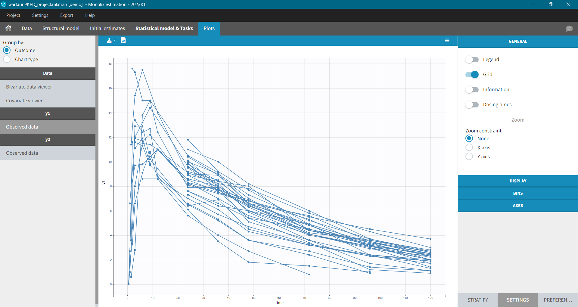
Settings in the right panel allow to adapt the plots display, full description is here.
General settings
General settings include: legend, display of grid, information about the data and dosing times.
Information adds a box with summary of the data and is recomputed for each subplot after splitting by a covariate. It includes:
- The total number of subjects
- The average number of doses per subject
- The total, average, minimum and maximum number of observations per individual.
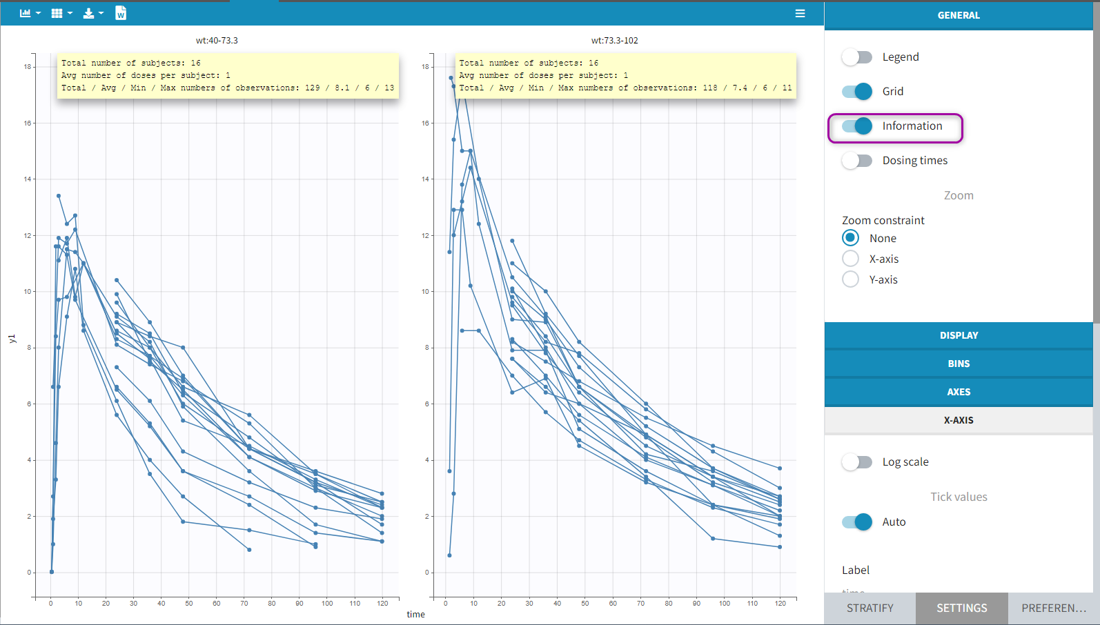
Option “dosing times” adds the individual dosing time as dashed vertical lines. You can make the lines always visible or only when you hover on individual data. Dosing times corresponding to doses with null amounts are not displayed.
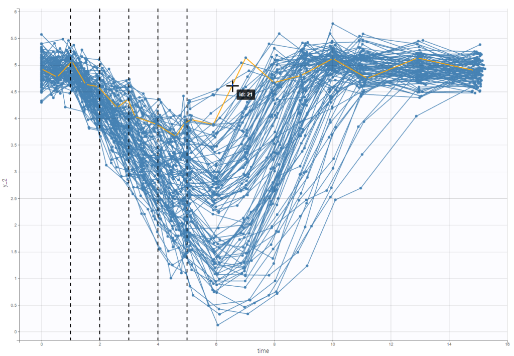
Display
You can display data as dots and lines (by default), or only as dots or only as lines, as in the figure below. Toggle “Mean” overlays a trend line on the plot, based on mean values of the observed data pooled in bins: arithmetic or geometric mean. Toggle “error bars” adds error bars as either the standard deviations or standard errors. The mean and error values can be displayed as fixed labels next to the bars, or as tooltips when hovering on a bar. If profiles contain censored data, these are by default displayed as red data points. Since version 2024, they can be hidden, if required, in the display section using the “Censored data” toggle. To avoid a possible distortion of the trend line, censored data can be excluded by disabling the “Use censored data” toggle in the statistics subsection
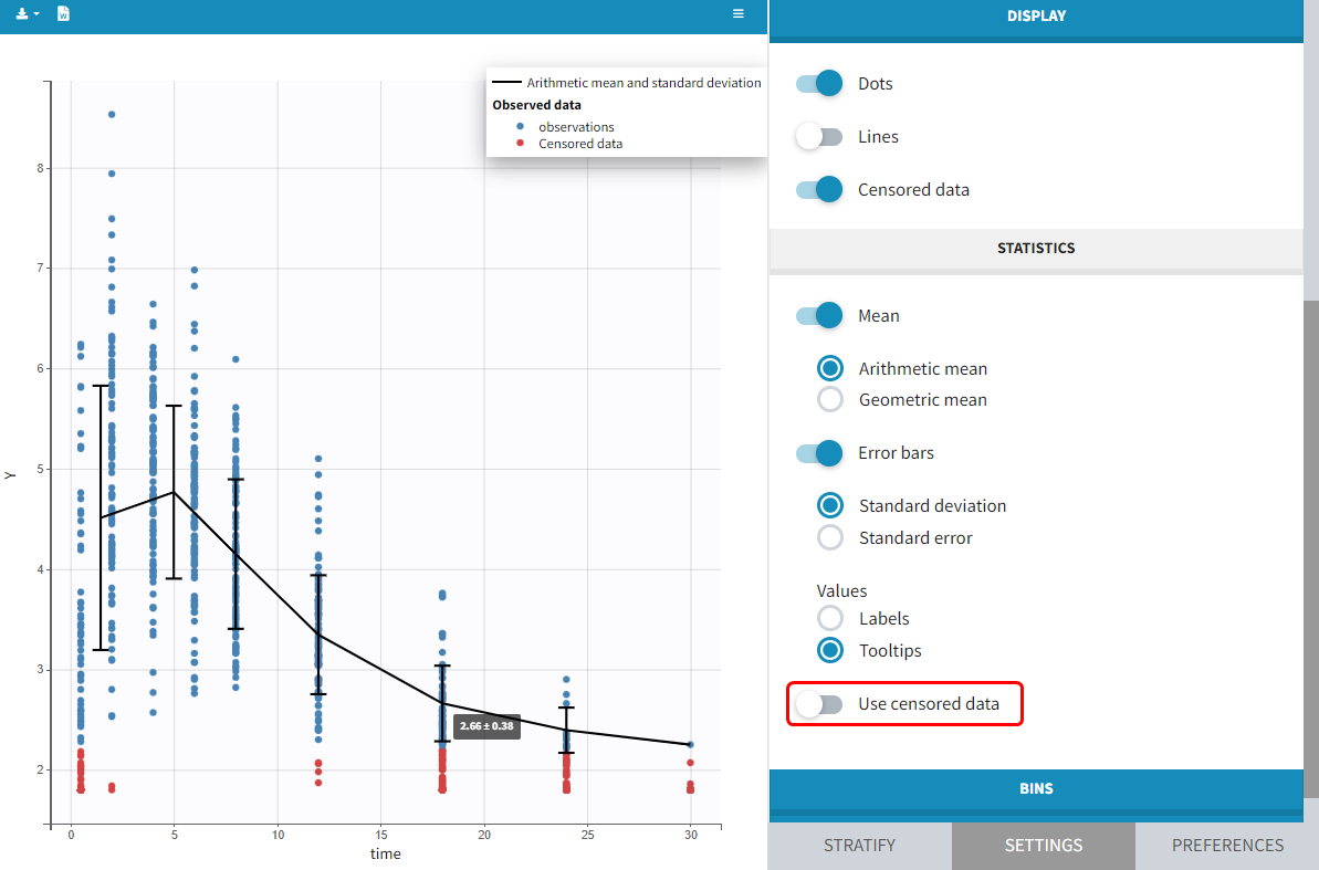
It is possible to display the mean curves, split by covariate, in a single plot. After split by a covariate, switch on the “Merged splits” option. In the example below, the mean curves of the two weight groups, which were in separate plots, are merged into a single plot. This feature is available for versions Monolix 2023 and above.
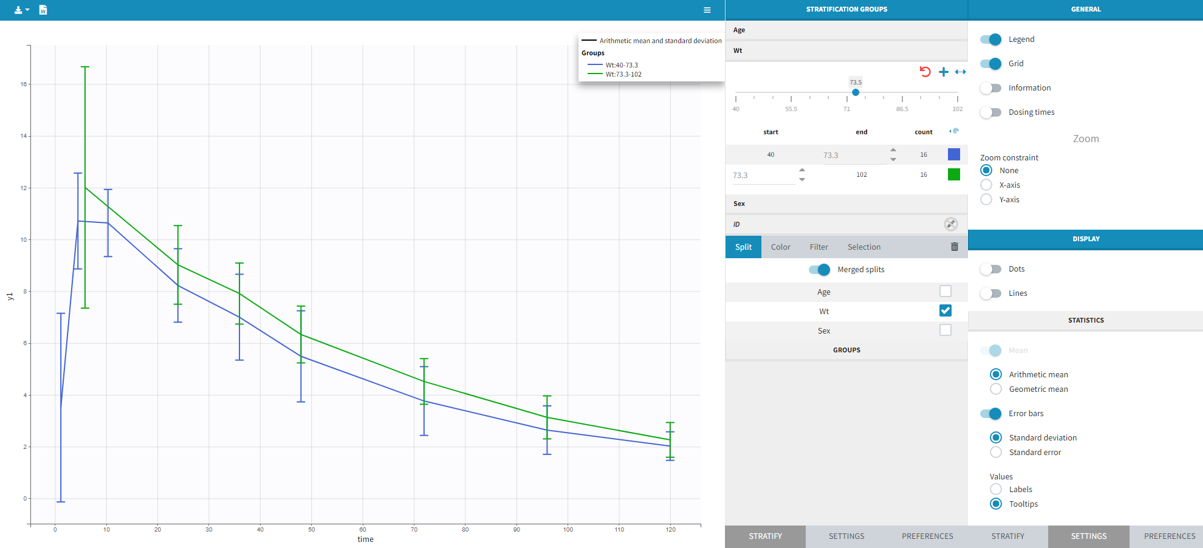
Bins
This section contains settings related to the definition of bins used in the computation of plot statistics. Toggle “bin limits” add vertical lines corresponding to the limits. In this section you can change the number of bins as well as binning criteria.
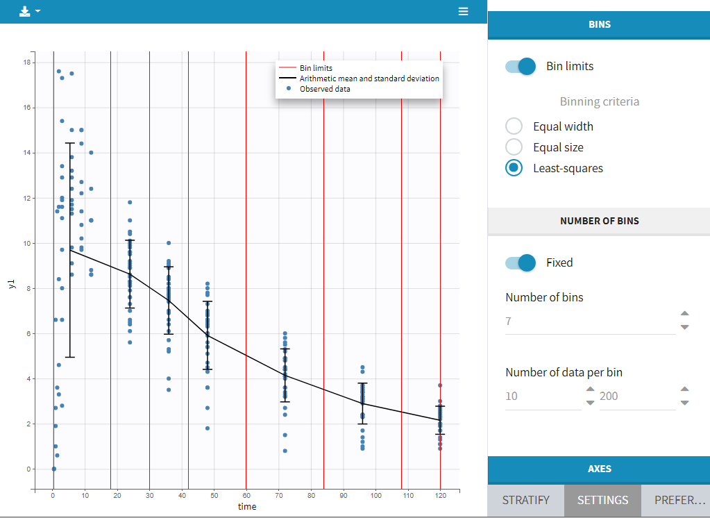
Axes
This section contains settings related to the display of X and Y – axis.
- Log scale toggle applies logarithm on a selected axis, for example to have a better evaluation of the elimination part.
- Nominal time option allows the nominal time to be displayed as time axis. This option is only available if nominal time has been tagged as such in the dataset (available in version 2024 and higher)
- Regressor option allows the values of the regressors tagged in the dataset to be displayed as x-axis (available in version 2024 and higher)
- Tick values “Auto” applies automatic axis ticks – if the toggle is enabled – or with a custom step – if the toggle is disabled.
- Label is an editable text displayed on each axis.
- Custom limits, when enabled, allows to choose the axis limits manually. They are applied to all subplots obtained by splitting by covariates.
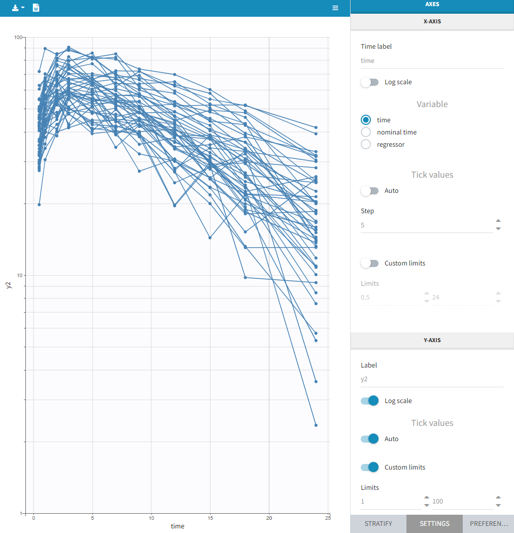
- Time after last dose toggle shows the spaghetti plot using on the x-axis time relative to the last dose (for Monolix version 2024 and higher). Below an example based on the demo project multidose_project.melxtran (Monolix demo folder 6.3)
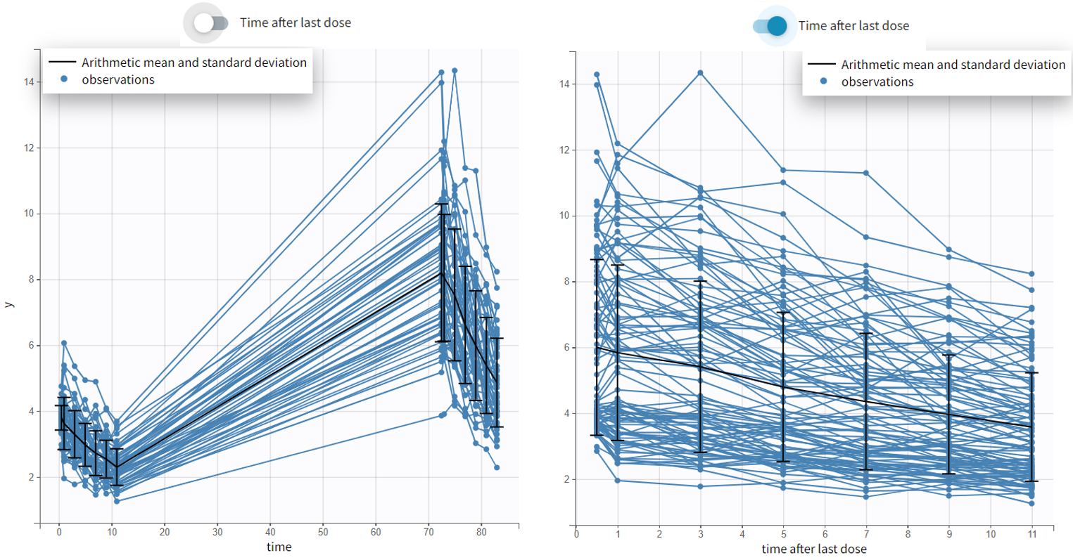 Discrete data
Monolix uses also count or categorical data, see here for detailed examples. Observed data can be shown as continuous, stacked or grouped. Example below shows the evolution of scores, which are categories describing anxious disorders, from the zylkene-data-set. The x-axis is time of measurements, while y-axis shows number of individuals in each category (different colors) at each time point. You can display the number of individuals for each category by hovering on it in the plot.
Settings, stratification and preferences work as for continuous data.
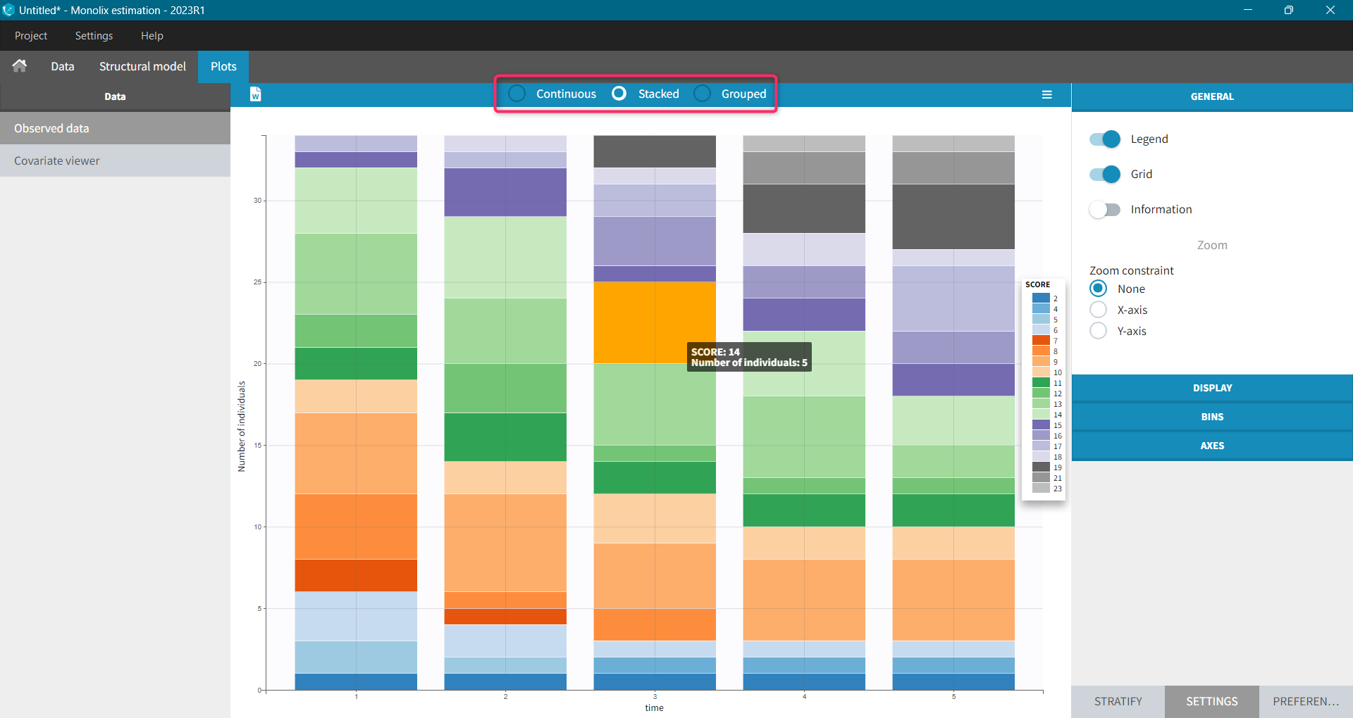
Time-to-event data
In Monolix, time-to-event data is displayed via a survival function, which describes the probability that an event happens after some time t. In general, this function is unknown and Monolix uses the non-parametric Kaplan-Meier estimator. It describes the probability that an individual survives until time t, knowing that it survived at any earlier time.
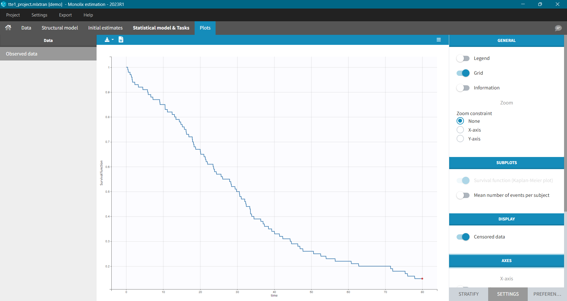
It is possible to display the Kaplan – Meier plot split by covariate in a single plot. After split by a covariate in the Stratify sub-tab, switch on the “Merged splits” option. In the example below, the curves of the four cell type groups, which were in separate plots, are merged into a single plot.
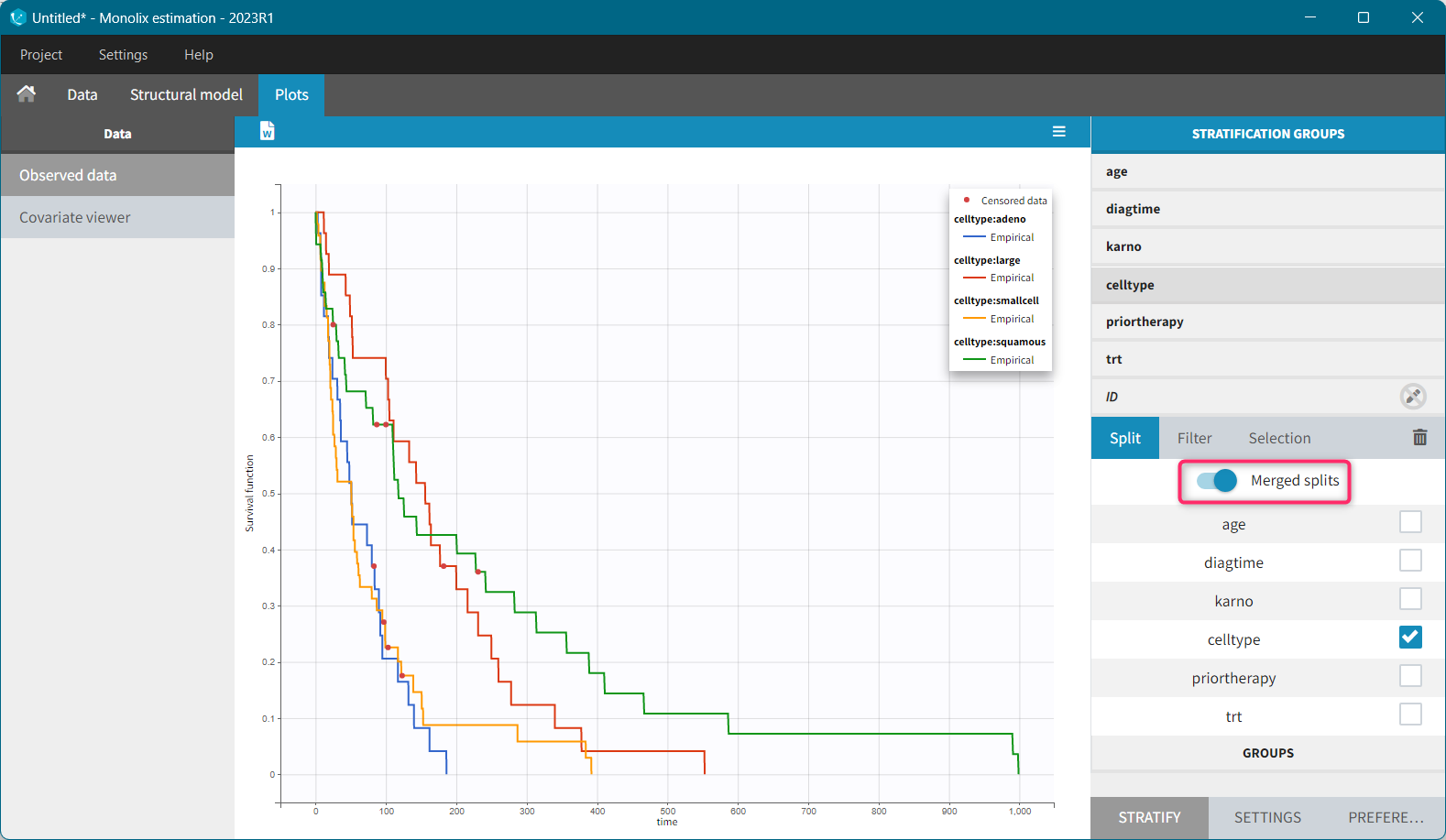
Kaplan – Meier estimator
For a single event data, the Kaplan-Meier estimator is given by the following formula
\( \hat{S}(t)=\sum_{i:t_i<t} \left(1-d_i/n_i\right),\)
where
- (t_i) – times before t, when at least one event occurred,
- (d_i) – number of events at the time (t_i),
- (n_i) – number of individuals at risk, that is who did not experience an event until (t_i).
The probability that an event occurs ((p_e)) is the ratio between the number of events that has occurred ((d_i)) and the total number of individuals at risk ((n_i)). The complement of it, ((1-p_e)), gives an estimation of the survival. For each time t the total number of individuals at risk changes, so the probabilities at all previous times (t_i), when at least one event occurred, are multiplied. It is similar to calculating the probability that a patient survives 2 days. It is a product of a probability that a patient survives the first day and a conditional probability that it survives the second day, knowing that it survived the first one.
Example:
A typical example of a time-to-event data set contains information about exact times when individuals experienced an event or when they left a study (drop-out). In the following, there are five individuals, who have two observations: time when the observation starts, which is 0 for all, and time of an event. If a patient leaves a study, then the time of a drop-out is given but instead of 1 in the column for the observation, there is 0. It indicates that this individual didn’t experience an event but survived until the drop-out time.The advantage of the Kaplan-Meier estimate is that it takes into account situations when not all individuals continue the study. At the next event time, such individuals are not counted as individuals at risk (they are not counted in the denominator (n_i)).
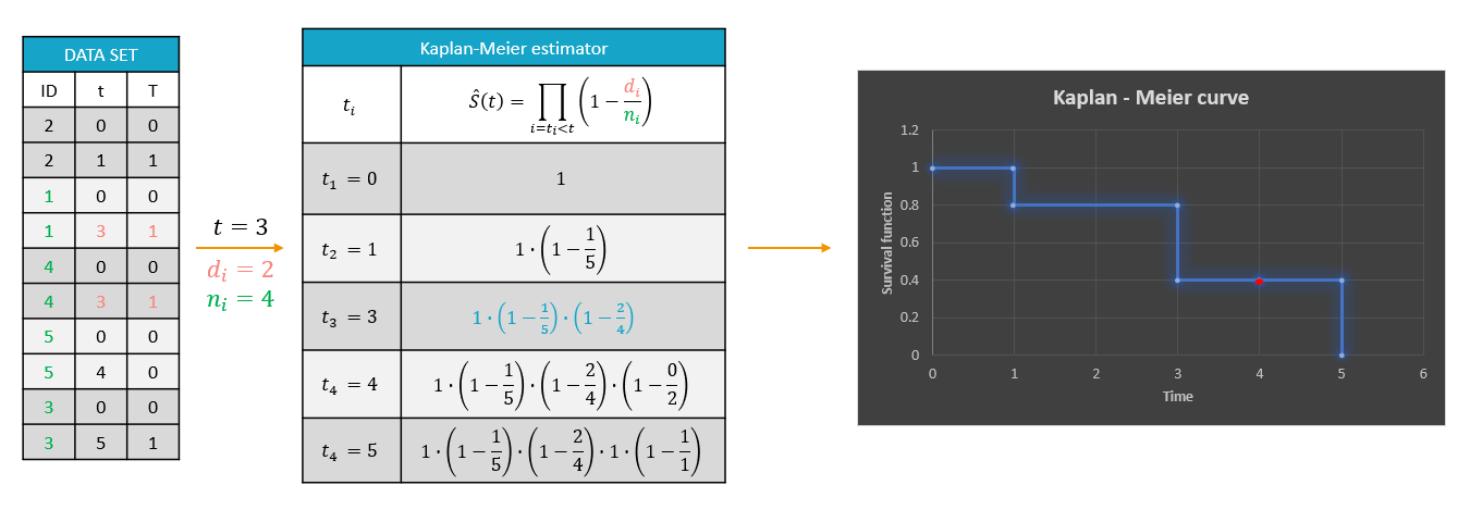
A study starts at time (t_1). There are no events, so (d_1=0) and the value of the survival curve is 1. Until the next event time at (t_2=1), the survival remains constant. Then, one individual experienced an event, so (d_2=1), and all individuals survived until that time, so (n_2=5). The result is that the probability to survive decreases by 0.2, which corresponds to the height of the jump at (t=1) in the plot. Then again, until the next event, survival remains constant. At time (t=3), there are two events. The number (n_3) counts now only 4 individuals – it has decreased by 1 due to the previous event. To get the final value probability at time 3is multiplied by all earlier probabilities. At (t=4) there is a drop-out. Patient 5 left the study and no event was registered. The survival curve remains constant, and the drop-out is marked in red. The Kaplan-Meier estimator takes into account this situations, because at the next event time (t=5), this individual is not counted as an individual at risk – denominator n will be smaller. At time (t=5), there is only one individual left, and one event, so the survival equals 0.
Remarks
- Kaplan-Meier estimator handles correctly information about individuals who left the study, but there is a bias when the exact times of events are unknown.
- In data visualization, Monolix assumes that all events are exactly observed. For example: assume that an observation period started at (t=0) and at (t=1) an event is marked by 1 in the column for the observation. It is impossible to distinguish in the dataset, without any other information, if the event was exactly at (t=1) or before. The same problem is when a time of the beginning of the study and time interval limits of an event are given. Just looking at the data set, an exact and interval censored event type are indistinguishable. In other words, not knowing when an event happened, Monolix assumes that it happened at the end of the censored interval.
Mean number of events.
The Kaplan-Meier estimator can be used also for the analysis of repeated events. The survival curve is estimated for each k-th event separately ( \hat{S}^{(k)}(t) = \sum_{i:t_i<t} \left(1-\frac{d^{(k)}i}{n^{(k)}_i}\right)), and is used to calculate the mean number of events per individual as a function of time (\hat{m}(t) = \sum{k} \left(1-\hat{S}^{(k)}(t)\right).) It can be visualized next to the Survival function by choosing this option from the Subplots settings:
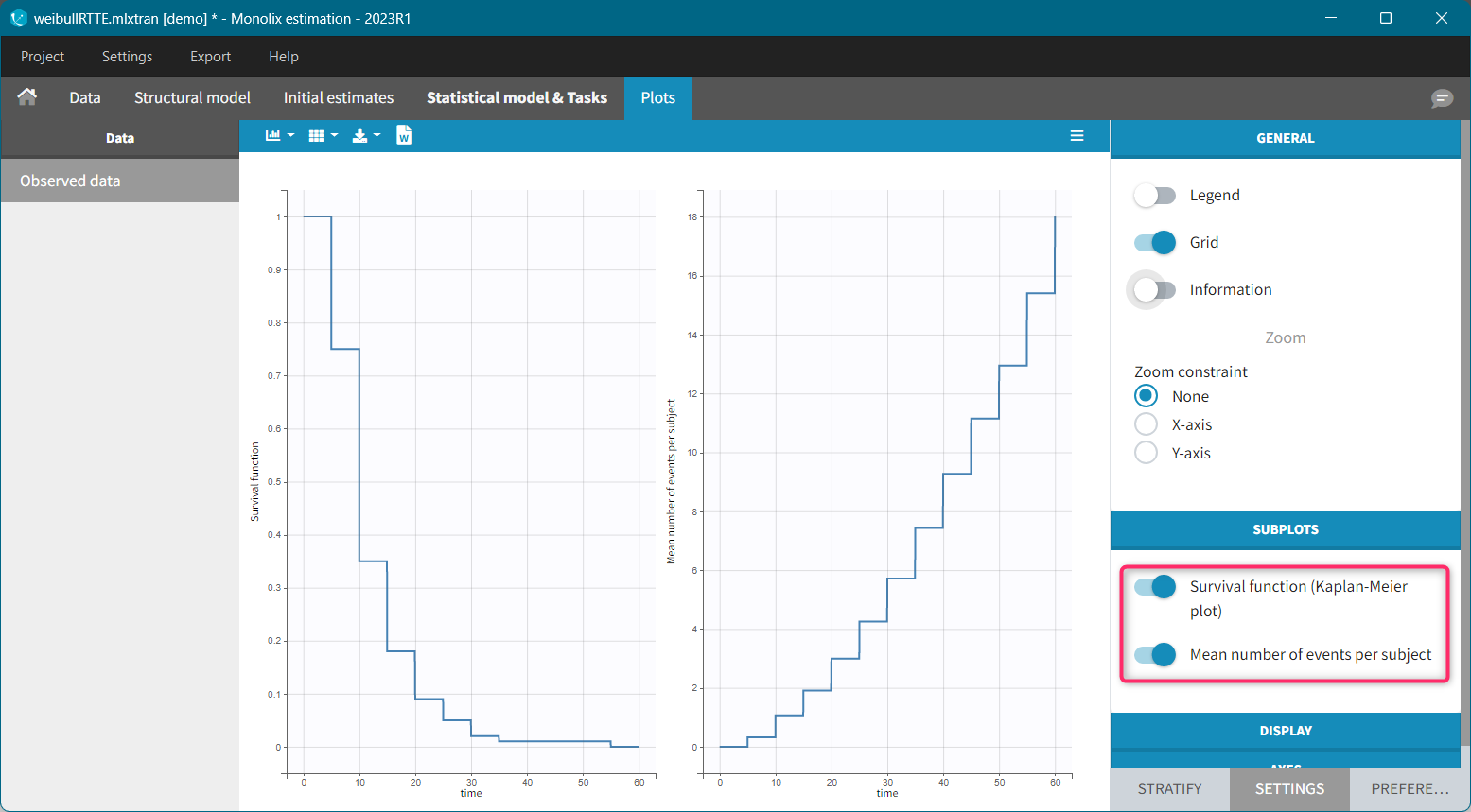
Settings
- General: Add/remove the legend, the grid, data information and dosing times; constrains on zoom
- Display: add/remove data dots, lines, mean and error bars
- Bins: display bin limits, binning criteria, number of bins
- Axes: Add/remove log-scale, modify labels, set tick values, set custom axis limits
- Stratify: Split, color and filter by covariates,
- Preferences: Add/remove elements or change colors and sizes for axes, observations, censored (BLQ) observations, highlighting.
Troubleshooting
If the Observed data plot is empty or with non-appropriate axis limits, follow the procedure below.
![]()
The problem appears after having clicked “Export > Export charts settings as default” on a previous project where the y-axis limits were different and this is now applied as default. It is possible to delete the default setting corresponding to the axis limits in the following way:
-
- Open the file C:/Users/<username>/lixoft/monolix/monolix2023R1/config/settings.default in a text editor
- Delete the following lines:
VPCContinuous\yInterval= ...
outputPlot\yInterval= ...
- Save the file
- Reopen your project
6.2.2.Covariate Viewer
It is possible to show the matrix of all the covariates as on the following figure:
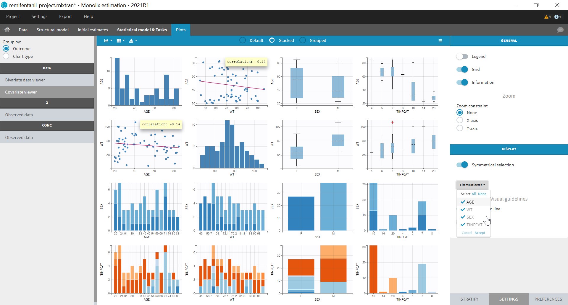
It is possible to display one covariate vs another one, selecting in the display panel which covariate to look at.
Here we display the age versus the wt and show the correlation coefficient as an information:

Categorical covariates w.r.t. other categorical covariates are displayed as a histogram (stacked or grouped),

and continuous covariates w.r.t. categorical covariates are displayed as a boxplot as below (“+” are outlier points below Q1-1.5*IQR (interquartile range) or above Q3+1.5*IQR):

Covariate statistics
Starting from the 2021 version, it is also possible to get the covariate statistics in a dedicated frame of the interface:
All the covariates (if any) are displayed and a summary of the statistics is proposed. For continuous covariates, minimum, median and maximum values are proposed along with the first and third quartile, and the standard deviation. For categorical covariates, all the modalities are displayed along with the number of each. Note the “Copy table” button that allows to copy the table in Word and Excel. The format and the display of the table will be preserved.
6.2.3.Bivariate Data Viewer
In case of several continuous outputs, one can plot one type of observation w.r.t. another one as on the following figure for the warfarin data set. The direction of time is indicated by the red arrow. Linear interpolation is used for observations of different types that are not at the same time.
Labels for x and y axes correspond to the observation names in the model for data types that are mapped to an output of the model, or observation ids used in the dataset for data types not captured by the model. It is possible to choose which observation id to display on X or Y axis in the settings panel on the right.
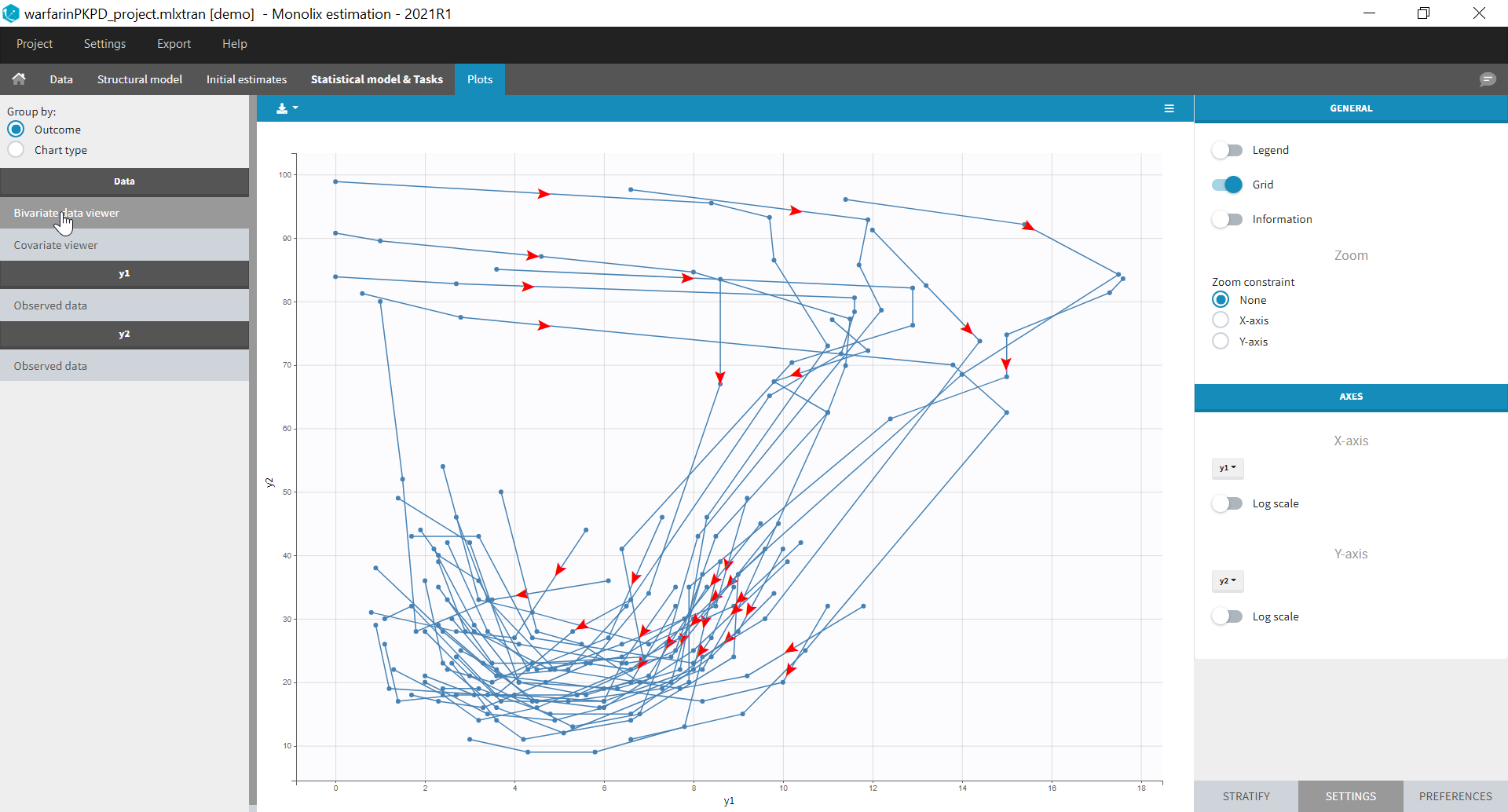
6.3.Model for the observations
6.3.1.Individual fits
Purpose
The figure displays the observed data for each subject, as well as two curves from simulations using the design and the covariates of each subject:
- the predicted profile given by the estimated population model (Population fits),
- the predicted profile given by the estimated individual model (Individual fits). If the EBEs and/or the conditional distribution tasks were performed, the user can choose either the conditional means or the conditional modes, estimated by MCMC, as estimators. Otherwise, approximations of the conditional means from SAEM are used.
This is a good way to see on each subject the validity of the model, and the actual fit proposed, as well as the inter-individual variability in the kinetics. It is possible to show the computed individual parameters on the figure. Moreover, it is also possible to display an individual predictive check: the median and a confidence interval for (
Examples
-
Individual fits and population fits
In the example below, the concentration for the theophylline data set is shown with simulations of a one-compartment model with first-order absorption and linear elimination. For each subject, the data are displayed with blue points along with the individual fit and population fit (the prediction using the estimated individual and population parameters respectively).
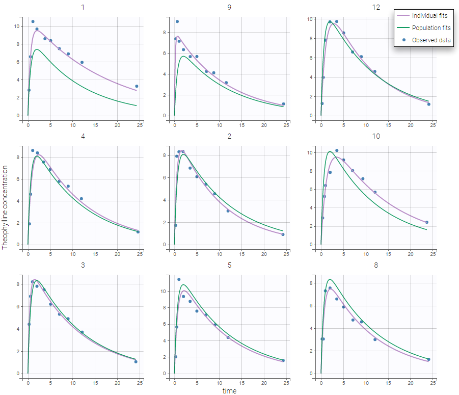
-
Individual parameters
Information on individual parameters can be used in two ways, as shown below. By clicking on Information (marked in green on the figure) in the General panel, individual parameter values can be displayed on each individual plot. Moreover, the plots can be sorted according to the values for a given parameter, in ascending or descending order (Sorting panel marked in orange). By default, the individual plots are sorted by subject id, with the same order as in the data set.
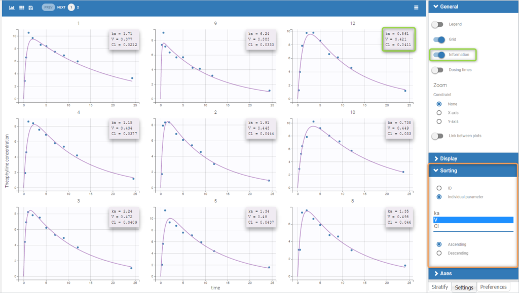
-
Individual predictive check
Individual predictive checks can be added to the plots: for each individual a prediction interval is computed based on multiple simulations with the population parameters and the design structure of this individual. The median line of the interval is also drawn. The interval allows to check whether the observed data are compatible with the population prediction, taking into account the inter-individual variability. The example below shows that the first subject in the theophylline data set show too much variability from the rest of the population to be correctly described by the population model.
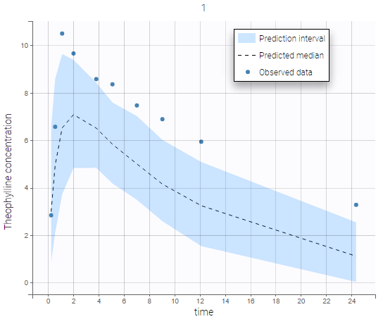
-
Dosing times
Dosing times can also be overlayed, which is useful to visualize the effect of doses on the prediction. As an example, the following figure shows the observations of an individual from the tobramycin data set along with the corresponding individual fit and multiple dosing times. Starting in version 2021R1 on, dosing times corresponding to doses with null amounts are not displayed.
-
Special zoom
User-defined constraints for the zoom are available. They allow to zoom in according to one axis only instead of both axes. Moreover, a link between plots can be set in order to perform a linked zoom on all individual plots at once. This is shown on the figure below with observations from the remifentanil example, and individual fits from a two-compartment model. It is thus possible to focus on the same time range or observation values for all individuals. In this example it is used to zoom on time on the elimination phase for all individuals, while keeping the Y axis in log scale unchanged for each plot.
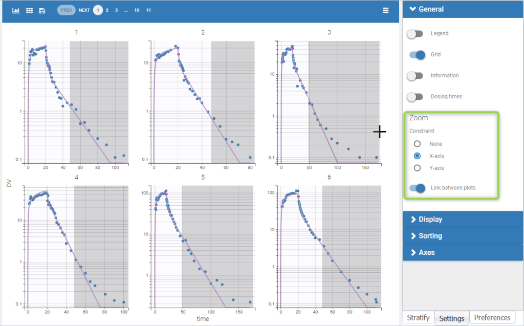
-
Censored data
When a data is censored, this data is different to a “classical” observation and has thus a different representation. We represent it as a bar from the censored value specified in the data set and the associated limit.
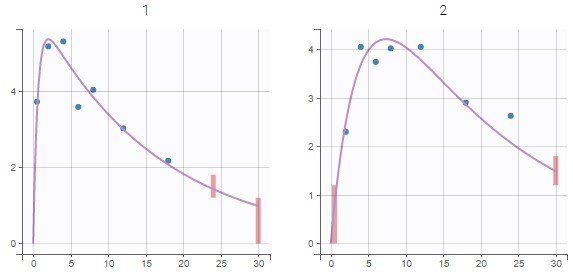
If there is no limit column then is goes to Infinity as in the following example. However, in any case, the user can choose the limit of the plot.
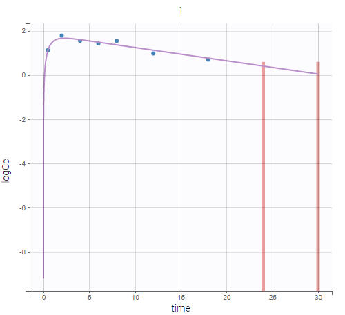
Settings
- Grid arrange. The user can define the number of subjects that are displayed, as well as the number of rows and the number of columns. Moreover, a slider is present to be able to change the subjects under consideration.
- General
- Legend: hide/show the legend. The legends adapts automatically to the elements displayed on the plot. The same legend box applies to all subplots and it is possible to drag and drop the legend at the desired place.
- Grid : hide/show the grid in the background of the plots.
- Information: hide/show the individual parameter values for each subject (conditional mode or conditional mean depending on the “Individual estimates” choice is the setting section “Display”).
- Dosing times: hide/show dosing times as vertical lines for each subject.
- Link between plots: activate the linked zoom for all subplots. The same zooming region can be applied on all individuals only on the x-axis, only on the Y-axis or on both (option “none”).
- Display
- Observed data: hide/show the observed data.
- Censored intervals [if censored data present]: hide/show the data marked as censored (BLQ), shown as a rectangle representing the censoring interval (for instance [0, LOQ]).
- Split occasions [if IOV present]: Split the individual subplots by occasions in case of IOV.
- Individual fits: Model prediction for each individual using the subject’s design and the individual parameters. The individual parameters can be the conditional mode or the conditional mean depending on the choice in the “Individual estimates” section.
- Population fits [if no covariates in the model]: Model prediction for each individual using the subject’s design and the population parameters.
- Population fits (individual covariates) [if covariates present in the model]: Model prediction for each individual using the subject’s design, the population parameters and the individual covariates values.
- Population fits (population covariates) [if covariates present in the model]: Model prediction for each individual using the subject’s design, the population parameters and the median covariates values (median from all individuals of the data set).
- Individual estimates [if EBEs task has run]: depending on the tasks that have been calculated, choice between conditional mode (given by EBEs task), conditional mean (approximation given by the population parameter estimated task) or conditional mean (given by the conditional distribution task).
- Individual predictive check: For each individual, 500 (see “number of simulations” in the PLOTS task settings) data sets are simulated using the individual’s design (dose and regressor values). The parameter values used for the simulation include the population parameter values, the individual covariate values and random effects sampled from the population distribution. The simulated data sets include residual errors. The prediction interval represents the interval containing 90% (see “level” setting) of the simulated data points. The predicted median is the median of all simulated data points. The individual predictive check allows to visualize the inter-individual variability (unexplained by covariates) and compare the population prediction to the individual observations.
- Sorting: Sort the subjects by ID or individual parameter values in ascending or descending order.
By default, only the observed data and the individual fits are displayed.
6.3.2.Observation versus Prediction
Purpose
This figure displays observations (\(y_{ij}\)) versus the corresponding predictions (\(\hat{y}_{ij}\)) computed using either the population parameters and covariate effects but random effects set to 0, or with the individual parameters. This figure is useful to detect misspecifications in the structural model. The 90% prediction interval, which depends on the residual error model, can be overlaid. Predictions that are outside of the interval are denoted as outliers. A high proportion of outliers suggest misspecifications in the model. Moreover, the distribution of the observations should be symmetrical around the corresponding predicted values.
- Population and individual predictions vs observations
- Visual guides
- Outliers proportion
- Individual estimates
- Highlight
- Log scale
- Settings
Population and individual predictions vs observations
The following example corresponds to the observations and predicted concentrations for the PK of warfarin, modeled by a one-compartment model with a first-order absorption and a linear elimination.On the left, predictions are made using the population parameters while on the right they correspond to the individual parameters. More points appear with the individual predictions: for each observation point, ten predictions are displayed, corresponding to ten simulated individual parameters.
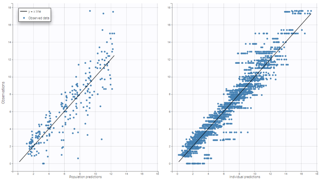
Visual guides
In addition to the line y = x, it is possible to display the 90% prediction interval, as well as a spline interpolation.
The 90% prediction interval represents the uncertainty of predictions due to the residual error model defined in the observation model. In the figure below, the shape of this interval can be seen for the four existing residual error models (constant, proportional, combined1, combined2) when the observation model is defined with a normal distribution:
The next figure corresponds to data that follow a log-normal distribution. The combination of constant error model and log-normal distribution corresponds to an exponential error model. Error models with a proportional term can cause numerical issues with the log-normal distribution for small observations because the error becomes very small as well.
Choosing an observation model with a logit-normal distribution for the data is useful to take into account bounded data. The figure below shows the shape of the prediction intervals for the different error models associated with data that follow a logit-normal distribution in [0.1-10]:
The prediction interval for the same example as above on the PK of warfarin characterizes a residual error model that combines a constant and a proportional term:
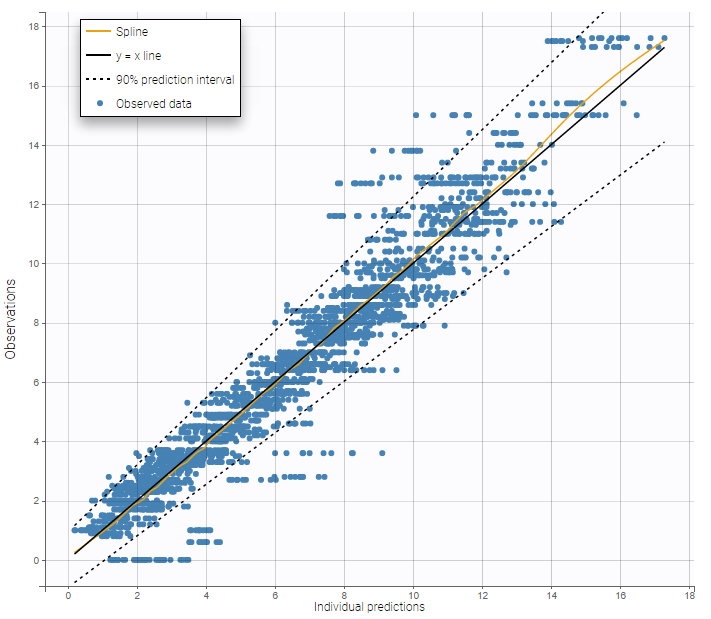
On the figure above it can be noted that several zero observations measured at low times correspond to nonzero predictions that fall outside the 90% prediction interval, and thus cannot be explained by the residual error. This could be explained by a delay between the administration and absorption of warfarin, therefore a model with a delayed absorption might fit better the data.
Outliers proportion
The outliers proportion can be displayed: it is the proportion of residuals outside the 90% prediction interval.
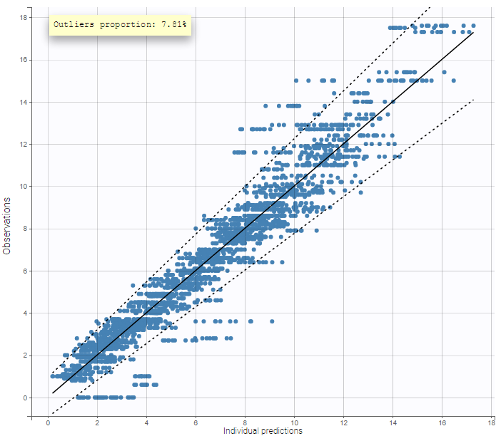
Individual estimates
As for all diagnosis plots based on individual parameters, it is possible to choose the individual estimates that are used to compute the plot of observations vs individual predictions, among the different estimates computed during the individual parameter estimation: conditional modes (EBEs) or means of the conditional distributions, or simulated individual parameters drawn from the conditional distributions (by default). In the latter case, each observation is associated with a set of individual predictions derived from a set of individual parameters simulated from the same individual conditional distribution. On the two figures below, one can compare the plot based on simulated parameters from the conditional distribution (top) and the same plot based on conditional modes (bottom).
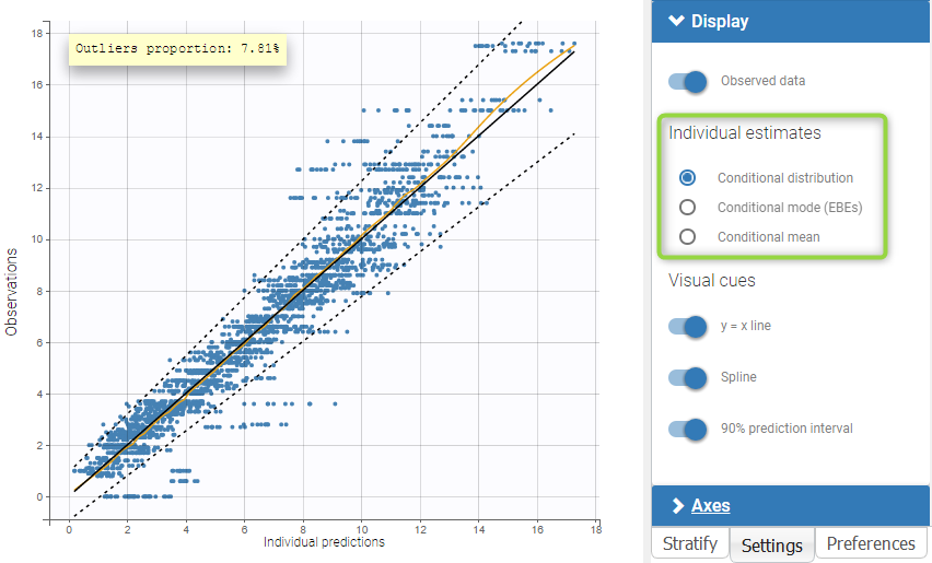
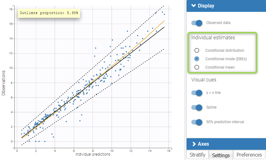
Highlight
As shown on the figures below, hovering on a point of observed data reveals the subject id and time corresponding to this point. All the points corresponding to this subject are highlighted in yellow. On the left, there are several predictions per observation, and the ten points corresponding to the hovered observation are indicated with a bigger diameter. On the right, there is only one prediction per observation, and all points corresponding to the same individual are linked with segments to visualize the time chronology.
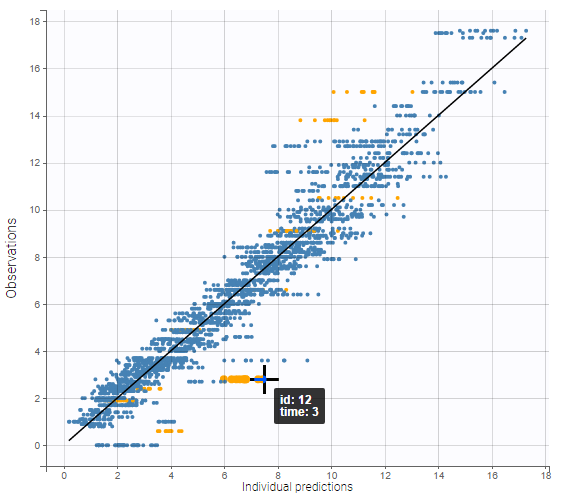
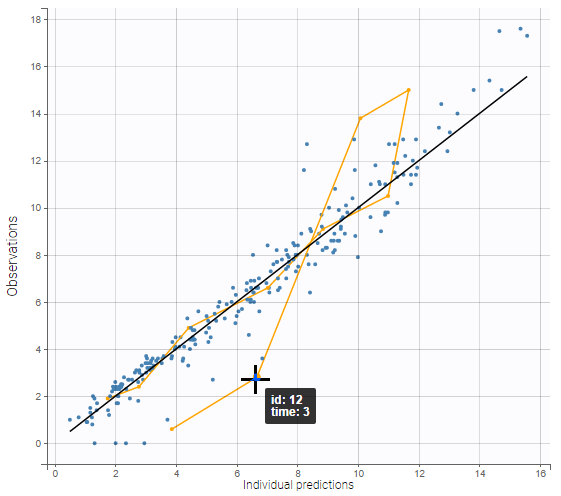
Log scale
A log scale is useful to focus on low observation values. It can be set for each axis separately or both together.
A second example below displays the predicted concentrations of remifentanil, modeled by a two-compartments model with a linear elimination. In this example, the log-log scale reveals a clear misspecification of the model: the small observations are under-predicted. These observations correspond to high times: this means that the elimination is not properly captured by the two-compartment model. A three-compartment model might give better results.
that here 10 predictions are displayed for each observation, corresponding to different simulated parameters drawn from the conditional distribution during the individual parameter estimation task.
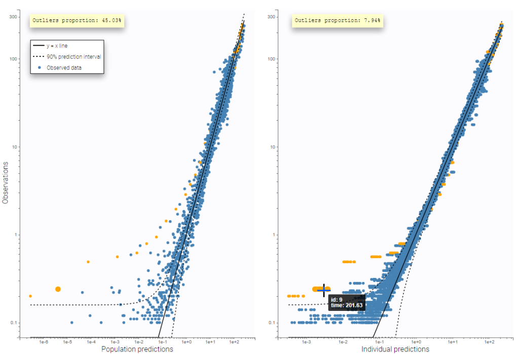
Settings
- General
- Legend and grid : add/remove the legend or the grid. There is only one legend for both plots.
- Outliers proportion: display/hide the proportion of points outside the 90% prediction interval.
- Subplots
- Population prediction: add/remove the figure with the comparison between the population predictions and the observations.
- Individual prediction: add/remove the figure with the comparison between the individual predictions and the observations.
- Display
- Observed data: Add/remove the points corresponding to pairs of observations and predictions.
- BLQ data : show and put in a different color the data that are BLQ (Below the Limit of Quantification)
- Individual estimates: select the estimates condition mean or mode, or simulated estimates from the conditional distribution (by default).
- Visual cues: add/remove visual guidelines such as the line y = x, a spline interpolation, and the 90% prediction interval indicated with dotted lines.
By default, only the individual predictions are displayed.
6.3.3.Scatter plot of the residuals
Purpose
These plots display the PWRES (population weighted residuals), the IWRES (individual weighted residuals), and the NPDEs (normalized prediction distribution errors) as scatter plots with respect to the time or the prediction.
The PWRES and NPDEs are computed using the population parameters and the IWRES are computed using the individual parameters. For discrete outputs, only NPDEs are used.
These plots are useful to detect misspecifications in the structural and residual error models: if the model is true, residuals should be randomly scattered around the horizontal zero-line.
Definition
Population Weighted Residuals \(\text{PWRES}_{ij}\)
\(\text{PWRES}_{ij}\) are defined as the normalized difference between the observations and their expected mean. Let \(y_i = (y_{ij}, 1 \leq j \leq n_i)\) be the vector of observations for subject i. The mean of \(y_i\) is the vector \(\mathbb{E}(y_i)=(\mathbb{E}(f(t_{ij};\psi_i), 1 \leq j \leq n_i)\). Let \( \textrm{V}_i\) be the \(n_j \times n_j\) variance-covariance matrix of \(y_i\). Then, the ith vector of the population weighed residuals \( \text{PWRES}_i = \{\text{PWRES}_{ij}, 1\leq j \leq n_i\} \) is defined by
$$\text{PWRES}_i = V_i^{-1/2}(y_i-\mathbb{E}(y_i))$$
The population residuals \((y_i-\mathbb{E}(y_i))\) are correlated within each individual. The population weighted residuals PWRES standardize and decorrelate the population residuals using the model-predicted variance-covariance matrix of observations \(V_i\).
\(\mathbb{E}(y_i) \) and \(V_i\) are not known in practice but are estimated empirically by Monte-Carlo simulation without any approximation of the model. In the formula above, \(y_i\) represents the observations from the dataset. \(\mathbb{E}(y_i)\) is calculated as the mean of simulated observations using individual parameters sampled from the population distribution to obtain the model prediction plus a sample from the residual error model. The number of simulated observations depends on the Plot task setting “Number of simulations”. \(V_i\) is calculated on the same simulated observations.
When the PWRES are plotted w.r.t the model prediction, the population prediction popPred (i.e with random effects eta equal to zero but keeping the covariate effects) are used on the x-axis.
Individual weighted residuals \(\text{IWRES}_{ij}\)
\(\text{IWRES}_{ij}\) are estimates of the standardized residual (\(\epsilon_{ij}\)) based on individual predictions, with \(g\) the function defining the residual error model:
$$\text{IWRES}_{ij} = \dfrac{ y_{ij}-f(t_{ij};\hat{\psi}_i)}{g(t_{ij};\hat{\psi}_i)}$$
If the residual errors are assumed to be correlated, the individual weighted residuals can be decorrelated by multiplying each individual vector \(\text{IWRES}_i = (\text{IWRES}_{ij} ; 1\leq j\leq n_i)\) by \(\hat{\text{R}}_i^{-1/2}\), where \(\hat{\text{R}}_i\) is the estimated correlation matrix of the vector of residuals \((\epsilon_{ij}; 1\leq j \leq n_i)\).
When the IWRES are plotted w.r.t the model prediction, the individual prediction using the conditional mode (EBEs), conditional mean or samples from the conditional distribution is used, depending on the choice of the “Individual estimates” in the settings panel on the right.
Normalized prediction distribution errors \(\text{NPDE}_{ij}\)
\(\text{NPDE}_{ij}\) are a nonparametric version of \(\text{PWRES}_{ij}\) based on a rank statistic. For any (i,j), let \(\text{F}_{ij} = \text{F}_{\text{PWRES}_{ij}}(\text{PWRES}_{ij})\) where \(\text{F}_{\text{PWRES}_{ij}}\) is the cumulative distribution function (cdf) of \(\text{PWRES}_{ij}\). NPDEs are then obtained from \(\text{F}_{ij}\) by applying the inverse of the standard normal cdf \(\Phi\).
In practice, one simulates a large number \(K\) of simulated data set \(y^{(k)}\) using the model, and estimate \(\text{F}_{ij}\) as the fraction of simulated data below the original data, i.e:
$$\hat{\text{F}}_{ij}=\frac{1}{K}\sum_{k=1}^K 1_{y_{ij}^{(k)}\leq y_{ij}^{\text{obs}}}$$
By definition, the distribution of \(\text{F}_{ij}\) is uniform on [0,1], we thus rather use \(\Phi^{-1}(\text{F}_{ij})\), which follows a standard normal distribution (with \(\Phi\) the cdf of the standard normal distribution). NPDEs are defined as an empirical estimation of \(\Phi^{-1}(\text{F}_{ij})\), i.e \(\text{NPDE}_{ij}=\Phi^{-1}(\hat{\text{F}}_{ij})\).
When the NPDE are plotted w.r.t the model prediction, the population prediction popPred (i.e with random effects eta equal to zero but keeping the covariate effects) are used on the x-axis.
Below is a correspondence table of the Nonmem and Monolix terms used for residuals:
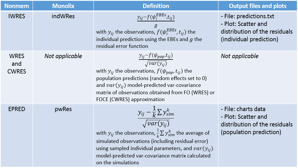
For count and categorical data:
FAQ: Is there no CWRES in Monolix? No, PWRES are given instead. They are defined with the same formula but are obtained with simulations rather than FOCE approximation, so without any approximation of the model. The PWRES in Monolix are equivalent to the EWRES in Nonmem.
Examples
In the following example, the parameters of a two-compartment model with iv unfusion and linear elimination are estimated on the remifentanil data set. One can see the PWRES, the IWRES and the NPDE w.r.t. the time (on top), and the prediction (at the bottom).
Since the points are clearly scattered unevenly around the horizontal zero-line, these plots suggest a misspecifcation of the structural model.
The corresponding distributions can be seen on this page.

It is possible to select some of the subplots to focus on, with the panel Subplots in Settings:

Presets
A number of element can be overlaid or hidden from the plots in the panel Display. Only the horizontal zero-line, representing the theoretical mean, is always displayed. Two presets with predefined selections of displayed elements are available: the first one called “Scatter” hides all elements except the points for residuals, while the second called “VPC” displays instead empirical and predicted percentiles for the residuals as lines, as well as prediction intervals as colored areas. This figure is detailed below.
 |
 |
|---|
Predictive checks
The preset “VPC” displays prediction intervals for the median, 10th and 90th percentiles, obtained with simulations of the residuals, as well as the empirical percentiles to compare the behavior of the model to the data. Residual points are hidden, but the trend is represented with a spline interpolation.
Misspecification in the structural model, the error model, and the covariate model can be detected by discrepancies between the observed percentiles and their prediction intervals, as can be seen for example on the plots of IWRES vs time and NPDE vs time below, with log-scale on the x-axis. Population residuals greatly depart from the data at all time points, while individual residuals show better predictions for low times only.
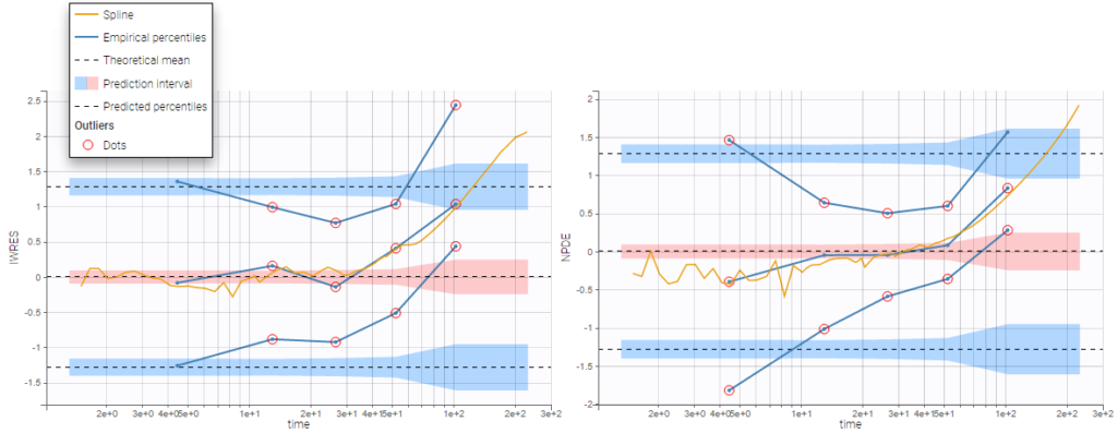
Outliers (empirical percentiles outside the prediction intervals) can be marked with red points or red areas:
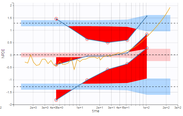
Comparing PWRES and NPDEs
NPDEs are quite similar to PWRES, but are simulation-based, and therefore account for the heterogeneity in study design by comparing the observations with their own distribution. NPDEs are thus displayed by default rather than PWRES.

Comparing IWRES and NPDEs
The IWRES are based on individual predictions, therefore the values on the X axis with respect to predictions are not the same as for NPDEs and PWRES, as can be seen on the plots below. If the tasks EBEs and Conditional distribution have been run, several different individual estimates are available to be used for the individual predictions. The next section shows how to choose the estimates.
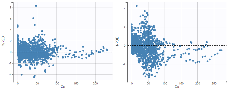
Preventing shrinkage in IWRES
The individual estimates used to compute the IWRES can be chosen in the Display panel:

By default, the individual estimates are drawn from the conditional distributions rather than coming from usual estimators such as conditional modes (EBEs) or conditional means. This choise is recommended in order to prevent shrinkage, a phenomenon that occurs when the individual data are not sufficiently informative with respect to one or more parameters. If overfitting occurs, IWRES computed from biased estimators might thus shrink toward 0.
Highlight
Hovering on a point highligths all the points from the same individual in yellow on all plots, and reveals the corresponding subject id and time. If the individual estimates selected in Display are the simulated condition distribution, each observation corresponds to a set of IWRES computed from a set of simulated individual parameters. When the observation is hovered, the points from this set are indicated with a bigger diameter.

If the individual estimates selected in Display are condition modes (EBEs) or conditional means, there is only one residual per observation, and all points corresponding to the same individual are linked with segments to visualize the time chronology.

Binning
As for VPC, data binning used to compute percentiles can be changed. Several strategies exist to segment the data: equal-width binning, equal-size binning, and a least-squares criterion. The number of bins can also be either set by the user, or automatically selected to obtain a good trade off.
On the three figures below where NPDEs are displayed with respect to log-scaled time, 5 bins are selected with equal width on the left, equal size in the center, and the least-squares criteria on the right. Observations are overlaid in light purple to visualize the data density in each bin. Equal width in particular shows low density for some bins, and result in a less informative plot for low times were data density is high.
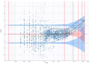 |
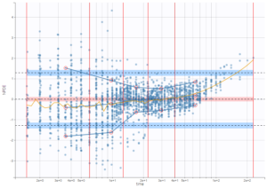 |
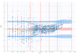 |
|---|
On the figure below, the number of bins for least-squares criteria is automatically set, allowing a more precise display.
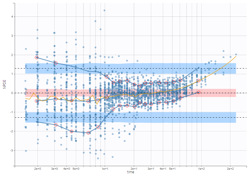
Censored data
The residuals for censored data appear in a different color. They are by default based on simulated observations that take into account the censoring interval.
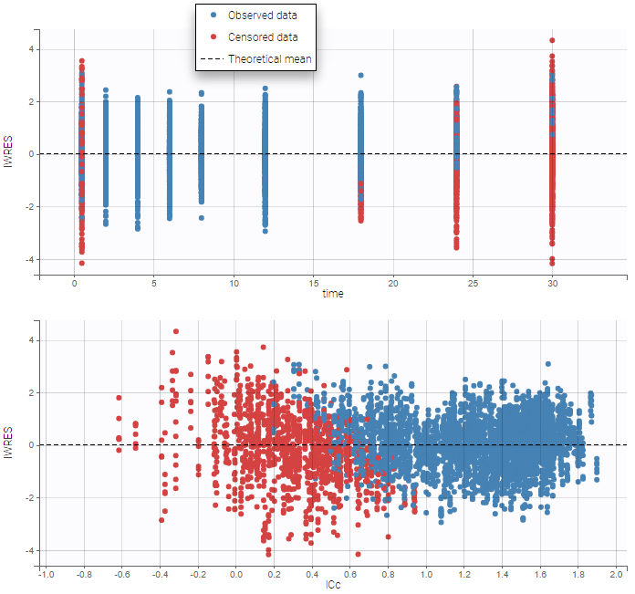
An option available in the panel “Display” can be used to select the method of calculation for the residuals corresponding to censored data: either based on simulated observations (by default), or based on LOQ (values from the observation column in the dataset).
Discrete data
For categorical or count data, only NPDEs are used. Here again, NPDEs correspond to the rank of each observation among a set of simulations based on the model. However, to prevent problems with discrete values, both observations and simulations are slightly perturbed with a uniform distribution before computing the ranks.
Settings
- Subplots
- Residuals
- Population residuals: Add/remove scatterplots for PWRES. Hidden by default.
- Individual residuals: Add/remove scatterplots for IWRES, using the individual parameter estimated using the conditional mode or the conditional mean. By default, individual parameters come from the conditional mode estimation.
- NPDE: Add/remove scatterplots for NPDE.
- X-axis
- time: Add/remove the scatterplots w.r.t. the time.
- prediction: Add/remove the scatterplots w.r.t. the prediction.
- Residuals
- Display
- Presets: apply the preselections of elements for scatter plots or VPC
- Residuals: Add/remove observed data.
- Censored data: Add/remove BLQ data (with a different color) if present.
- Empirical percentiles: Add/remove empirical percentiles for the 10%, 50% and 90% quantiles.
- Predicted percentiles: Add/remove theoretical percentiles for the 10% and 90% quantiles.
- Prediction interval: Add/remove prediction intervals given by the model for the 10% and 90% quantiles (in blue) and the 50% quantile (in pink), with user-defined level (by default, 90).
- Outliers: Add/remove dots or areas to mark outliers.
- Individual estimates: Choose the individual estimates among conditional modes (EBEs), conditional means (computed with SAEM), or simulated parameters from the conditional distributions.
- Calculations – linear interpolation: Choose the display for prediction intervals: by default linear interpolation is used, otherwise the display is piecewise.
- Calculations – Use censored data: Choose the display for censored data: by default simulated BLQ observations are used, otherwise the LOQ from the observation column in the data set can be used.
- Visual cues: Add/remove spline interpolation.
- Bins
- Bin values: Add/remove vertical lines on the scatterplots to indicate the bins.
- Binning criteria: Choose the bining criteria among equal width (default), equal size or least-squares.
- Number of bins: Choose a fixed number of bins or a range, with the range for the number of data points per bin.
6.3.4.Distribution of the residuals
Purpose
These plots display the empirical distributions of the residuals: the PWRES (population weighted residuals), the IWRES (individual weighted residuals), and the NPDEs (normalized prediction distribution errors) for continuous outputs, together with the standard Gaussian probability density function and cumulative distribution function.
If the model is true, the PWRES, IWRES and NPDEs should behave as independent standardized normal random variables. These plots are thus useful to detect misspecifications in the structural and residual error models.
Example
In the following example, the parameters of a two-compartment model with iv unfusion and linear elimination are estimated on the remifentanil data set.
Below, one can see on top the comparison between the empirical and theoretical probability density function (PDF) of the PWRES, IWRES and NPDE, and at the bottom the comparison between the empirical and theoretical cumulative distribution function (CDF).
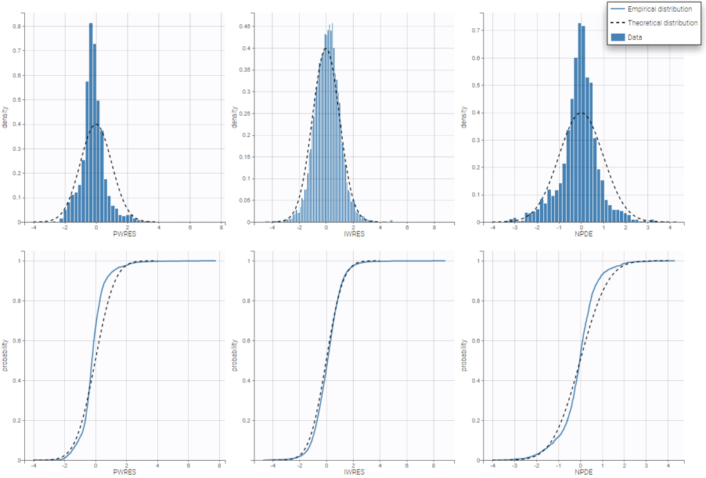
The corresponding scatter plots can be seen on this page.
Settings
By default, all the residuals and all the plots are displayed.
- Subplots
- Residuals: choose the plots to display according to residuals
- Population residuals: PWRES
- Individual residuals: IWRES, using the individual parameter estimated using the conditional distribution, the conditional mode, or the conditional mean.
- NPDE
- X-axis
- PDF: Probability density function of residuals and empirical distribution as histograms.
- CDF: Theoretical and empirical cumulative distribution functions.
- Residuals: choose the plots to display according to residuals
- Display
- Individual estimates: choose the estimator for individual parameters as parameters drawn from the conditional distributions. or the modes or means of the conditional posterior distributions.
6.4.Model for the individual parameters
6.4.1.Distribution of the individual parameters
Purpose
This figure can be used to compare:
- the empirical distribution of the individual parameters, estimated with the conditional means, the conditional modes, or simulated from the conditional distributions,
- the theoretical distribution defined in the statistical model, with the estimated population parameter.
Further analysis such as stratification by covariate or shrinkage assessment can be performed and will be detailed below.
PDF and CDF
In the warfarinPK_project, several parameters are estimated. It is possible to display the theoretical distribution and the histogram of the empirical distribution as proposed below.
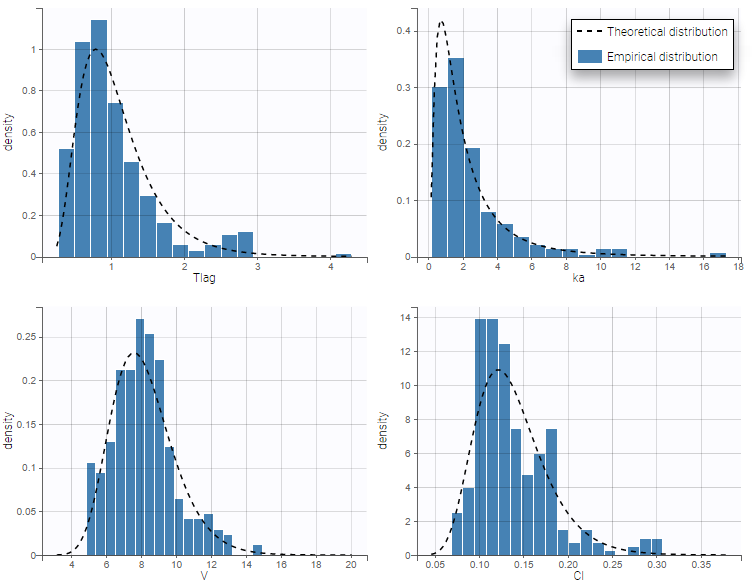
The distributions are represented as histograms for the probability density function (PDF). Hovering on the histogram also reveals the density value of each bin as shown on the figure below
Notice that the theoretical pdf is a pure log-normal distribution. However, in case of covariate use with the parameters, it is not a pure log-normal but rather a combinaison of log-normal distribution. If for example, on set the SEX covariate on the parameter V, a parameter beta_V_SEX_1 is created and the individual parameter distribution becomes as the following.
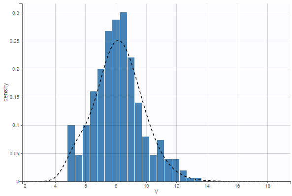
Cumulative distribution functions (CDF) is proposed too.
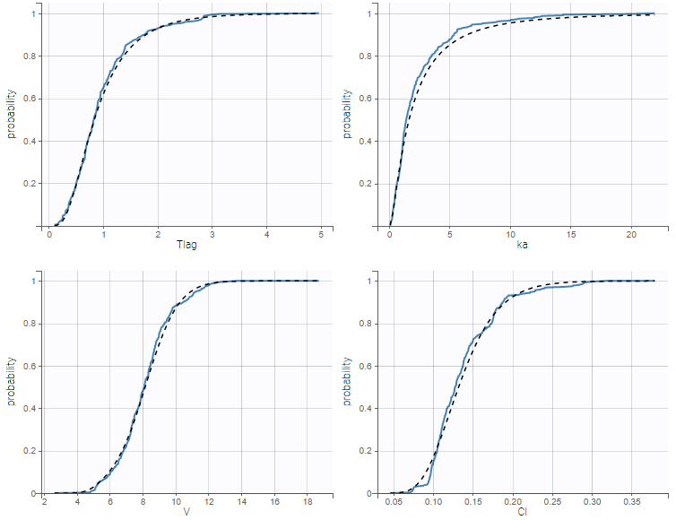
Again, overlaying the plots display the information concerning the parameter value and its empirical and theoretical cdf.
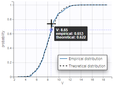
Getting away with shrinkage using simulated individual parameters
If the data does not contain enough information to correctly estimate some individual parameters, the individual estimates coming from the means or the modes of the individual conditional distributions shrink towards the same population value (respectively the mean or the mode of the population distribution of the parameter), a phenomenon known as shrinkage. For a parameter \(\psi_i\) that is a function of a random effect \(\eta_i\), this phenomenon can be quantified by defining the \(\eta\)-shrinkage as:
$$\eta\text{-shrinkage} = 1 -\frac{sd(\hat{\eta_i})}{\hat{\omega}} $$
where \(\text{sd}\left(\hat{\eta}_i\right)\) is the empirical standard deviation of the estimated random effects \(\hat{\eta}_i\)’s. The \(\hat{\eta}_i\) can be calculated from the EBEs, the conditional mean or the samples from the conditional distribution. Typically, the shrinkage is reported using the EBEs. Previously, in Monolix version 2023 and earlier, shrinkage was defined based on the variance as \(\eta\text{-shrinkage} = 1 -\frac{Var(\hat{\eta_i})}{\hat{\omega^2}}\). It is possible to display the shrinkage value on top of the histograms, as seen below for the conditional mode (EBEs):
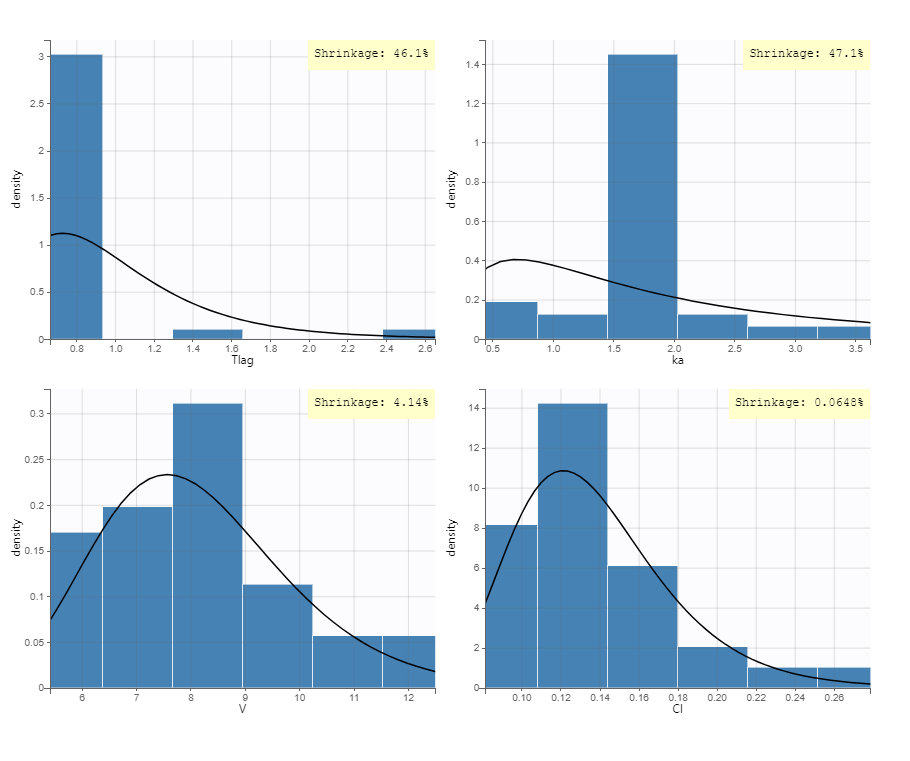
Selecting the “Conditional distribution” option instead for the individual estimates uses individual parameters drawn from the conditional distribution, simulated using MCMC sampling. This method is recommended as it results in unbiased estimators that are not affected by possible shrinkage, and leads to more reliable results. For more details see the page Understanding shrinkage and how to circumvent it.
In the same example, using the conditional distribution instead of the conditional mode reduces shrinkage, as can be seen below.
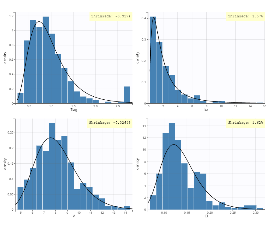
The following table shows the shrinkage calculation (in %) for all methods. The shrinkage is large for Tlag and ka when using the EBEs, which means that the individual data is not reach enough to reliable estimate the EBEs for Tlag and ka. The close to zero shrinkage value when using the samples from the conditional distribution shows that the samples from the conditional distributino are well spead over the population distribution, as expected.
| Method\Parameters | Tlag | ka | V | Cl |
|---|---|---|---|---|
| Conditional mean | 43.45 | 42.3 | 3.18 | 0.15 |
| Conditional mode (EBEs) | 46.07 | 47.11 | 4.14 | 0.065 |
| Conditional distribution | -0.317 | 1.57 | -0.26 | 162 |
Example of stratification
It is possible to stratify the population by some covariate values and obtain the distributions of the individual parameters in each group. This can be useful to check covariate effect, in particular when the distribution of a parameter exhibits two or more peaks for the whole population. On the following example, the distribution of the parameter k from the same example as above has been split for two groups of individuals according to the value of the continuous covariate AGE, allowing to visualize two clearly different distributions.

Settings
- General: add/remove the legend, the grid, and the shrinkage in %.
- Display
- Empirical: add/remove histogram of empirical distribution.
- Theoretical: add/remove curve of theoretical distribution.
- Distribution function: The user can choose to display either the probability density function (PDF) as histogram or the cumulative distribution function (CDF).
- Individual estimates: The user can define which estimator is used for the definition of the individual parameters.
Simulated individual parameters are used by default, otherwise the conditional mode is the default estimation if it has been computed with the “Individual parameters estimation” task.
6.4.2.Distribution of the random effects
Purpose
This plot displays the distribution of the standardized random effects with boxplots or with histograms. Since random effects should follow normal probability laws, it is useful to compare the distributions to standard Gaussian distributions.
Example
In the following example, one can see the distributions of two parameters of a two-compartment bolus model with linear elimination, estimated on the tobramycin example. On the left, the distributions are represented as boxplots, in the middle as histograms for the probability density function (PDF), and on the right as cumulative distribution functions (CDF). In each case, marks to compare the results to standard Gaussian distributions are overlaid: dotted horizontal lines indicate the interquartile interval of a standard Gaussian distribution for the boxplots, and black curves represent the PDF and CDF of a standard Gaussian distribution.
In boxplots, the dashed line represents the median, the blue box represents the 25th and 75th percentiles (Q1 and Q3), and
the whiskers extend to the most extreme data points, outliers excluded. Outliers are the points larger than Q1 + w(Q3 – Q1) or smaller than Q1 – w(Q3 – Q1) with w=1.5. Outliers are shown with red crosses.
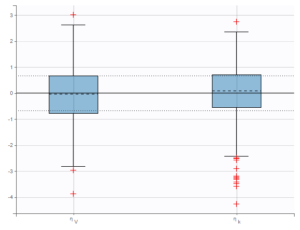 |
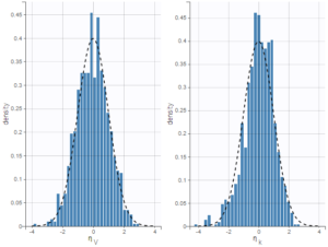 |
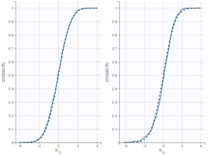 |
|---|
On the figure below, the individuals have been split into two groups according to the value of the continuous covariate CLCR. One can notice differences on the boxplots for the distributions of random effects between both groups, in particular for the parameter k.
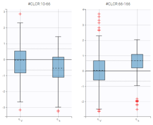
Shrinkage
When there is not enough data to well-estimate individual parameters, individual estimates based on the conditional mean or mode (rather than the entire conditional distribution) have a tendency to shrink towards the population parameter estimate. For the distribution of the standardized random effects, shrinkage leads to bias showing less than the true variation if the individual estimates are shown using the conditional mean or conditional mode rather than the conditional distribution in this case. The shrinkage can be displayed in the plot by toggling “information” in general settings. For more details see the page Understanding shrinkage and how to circumvent it.
Settings
- General: add/remove the grid and the shrinkage in %.
- Display
- Distribution function. The user can choose which type of plot is used to represent the distributions of the random effects: boxplots, pdf (probability density function) or cdf (cumulative distribution function).
- Individual estimates. The user can define which estimator is used for the definition of the individual parameters and thus for the random effects (conditional mean, conditional mode, or conditional distribution)
- Visual cues: If boxplot has been selected, the user can choose to add or hide dotted lines to mark the median or quartiles of a standard Gaussian distribution.
By default, the distributions of simulated random effects are displayed as boxplots.
Standarized random effects in case of IOV
Starting from the 2019 version, in case of IOV and if the conditional distribution is computed, we propose to display the standarized random effect by level of variability. In the presented example, we put IOV on both ka and V parameters. Thus, in the plot, we proposed to display the several levels of variability for all the parameters. We can then display the standarized random effects for
- the ID level,
- the OCC level (where only the parameters with variability on this level are displayed)
- the ID+OCC level corresponding to the addition of the levels
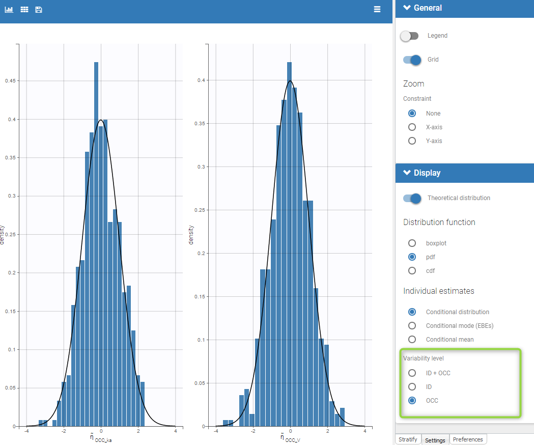
6.4.3.Correlation between the random effects
Purpose
This plot displays scatter plots for each pair of random effects. It allows to identify correlations between random effects, which can then be introduced in the models for the probability distributions for the individual parameters.
Example
In the following example, one can see pairs of random effects estimated for all parameters of a one-compartment model with delayed first-order absorption and linear elimination estimated on the PK of warfarin data set. The estimators for random effects have been simulated from conditional distributions of individual random effects.
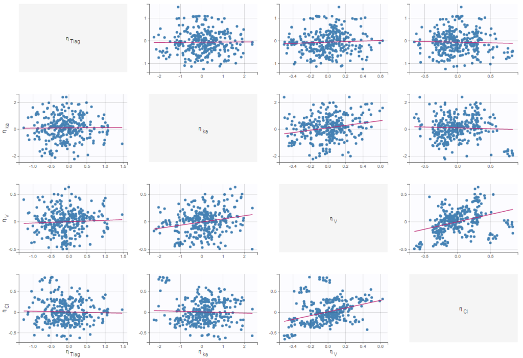
Visual guidelines
In addition to regression lines, Pearson correlation coefficients can been added to see the correlation between random effects, as well as spline interpolations.
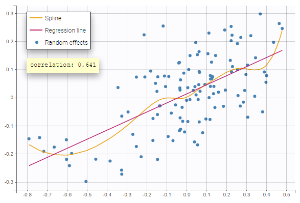
Selection
It is possible to select a subset of random effects, whose pairs of correlations are then displayed, as shown below. In the selection panel, a set of contiguous rows can be selected with a single extended click, or a set of non-contiguous rows can be selected with several clicks while holding the Ctrl key.
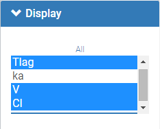
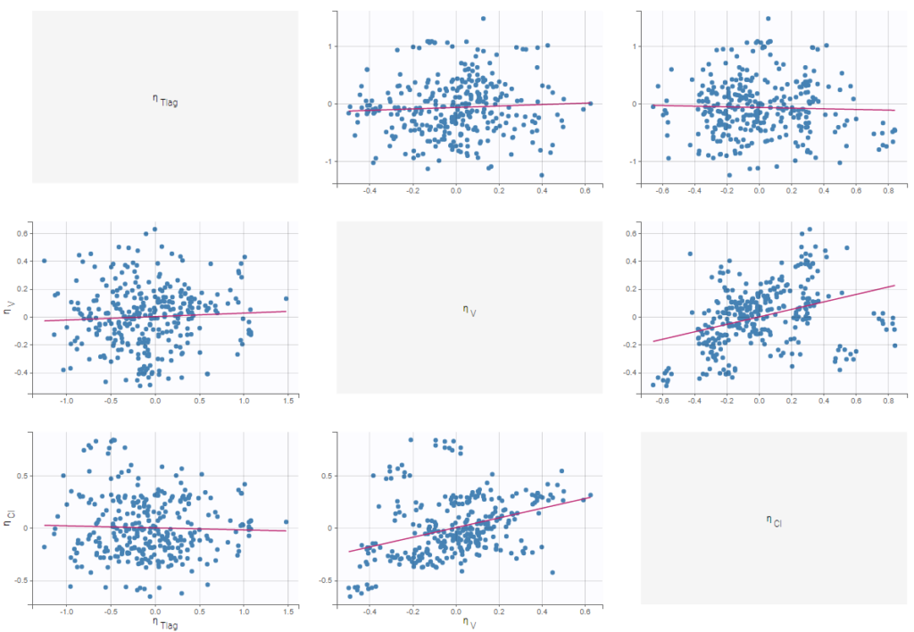
Highlight
Similarly to other plots, hovering on a point provides information on the corresponding subject id, and highlights other points corresponding to the same individual, if multiple individual parameters have been simulated by sampling the conditional distribution.
On the figure below, we can see the same plot with only one parameter value per individual (left) or ten values (right). Notice that the correlation coefficient is more reliable when multiple parameters are available, as they take into account the uncertainty of individual parameters.
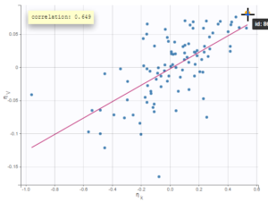 |
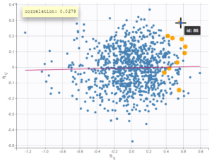 |
|---|
Stratification: coloring and filtering
Stratification can be applied by creating groups of covariate values. As can be seen below, these groups can then be colored (left) or filtered (right), allowing to check the effect of the covariate on the correlation between two parameters. The correlation coefficient is updated according to the filtering.
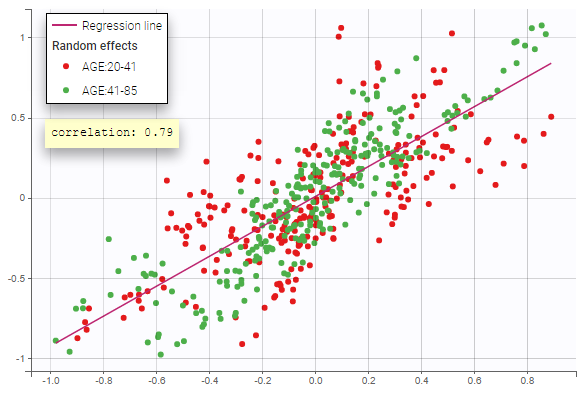 |
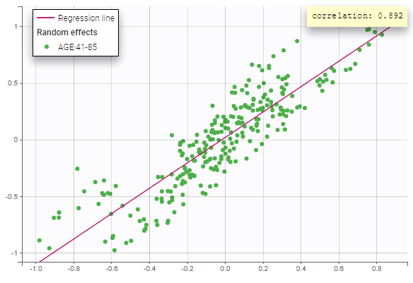 |
|---|
Settings
- General
- Legend and grid : add/remove the legend or the grid. There is only one legend for all plots.
- Correlation: display/hide the correlation coefficient associated with each scatter plot.
- Display
- Selection. The user can select some of the parameters to display only the corresponding scatter plots. A simple click selects one parameter, whereas multiple clicks while holding the Ctrl key selects a set of parameters.
- Individual estimates. The user can define which estimates are used for the definition of the individual parameters and thus for the random effects (conditional mean, conditional mode, simulated parameters)
- Visual cues. Add/remove the regression line or the spline interpolation.
By default, all scatter plots are proposed with simulated individual parameters.
Display in case of correlation in the statistical model
Starting from the 2019 version, when there is correlation in the statistical model, we propose to see the decorrelated random effects in order to see if some correlation remains. In that case, there is an option in the display to switch between the random effects and the decorrelated random effects as can be seen on the following figure. The methodology behind the calculation can be found here. The formula to calculate the decorrelated random effects \(\hat{\eta}_i\) from the random effects \(\eta_i\) and the estimated variance-covariance of the random effects \(\Omega\) is:
\(\hat{\eta}_i=\Omega^{-1/2}\times \eta_i \)
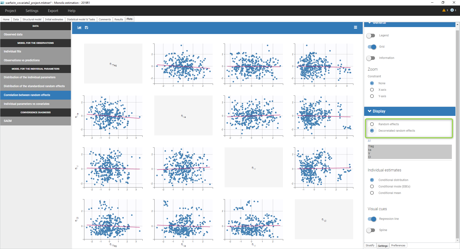
Display in case of IOV
Starting from the 2019 version, in case of IOV and if the conditional distribution is computed, we propose to display the by level of variability as can be seen in the following figure.
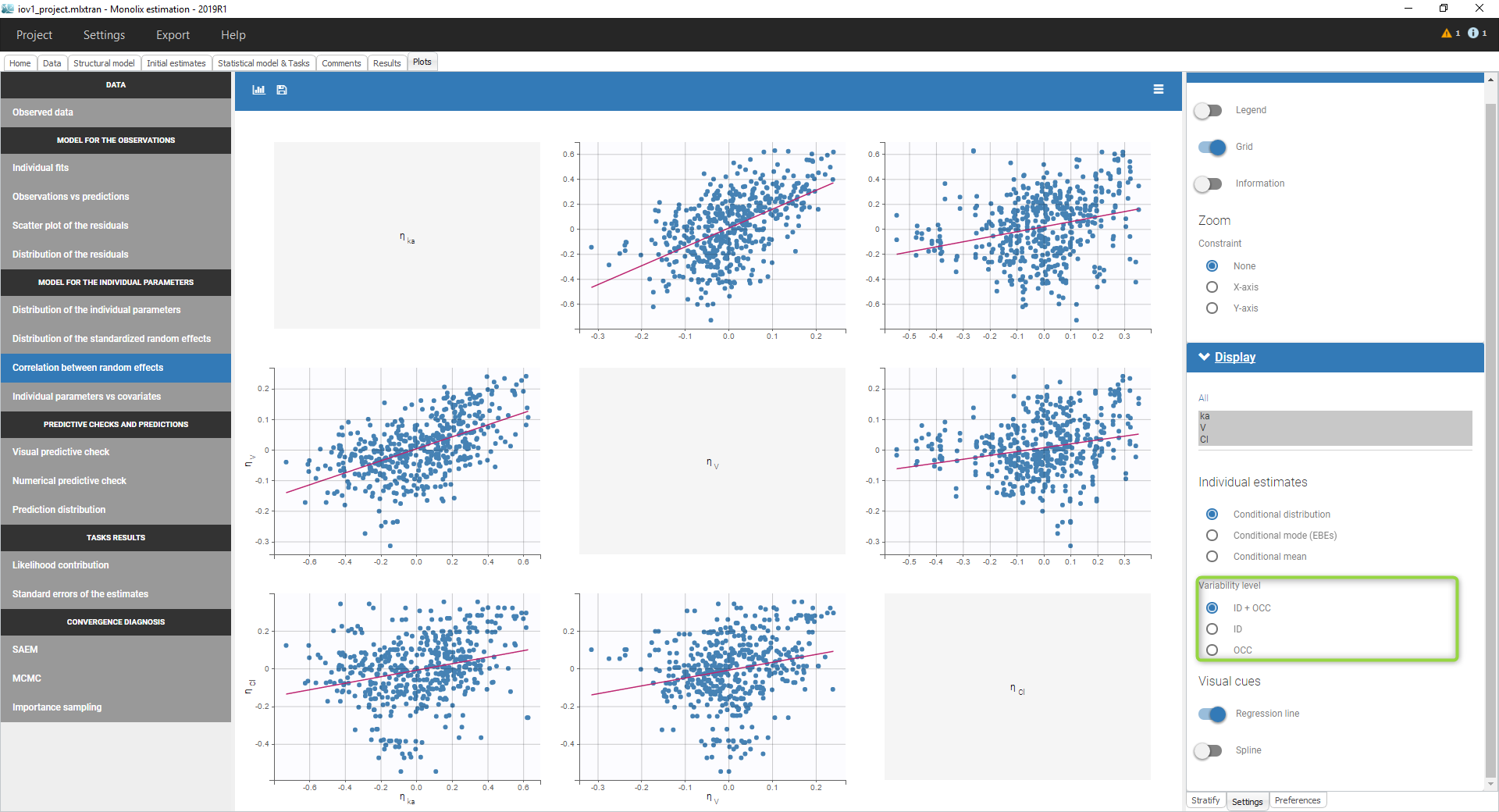 We can then display the correlation of the random effects for
- the ID level,
- the OCC level (where only the parameters with variability on this level are displayed)
- the ID+OCC level corresponding to the addition of the levels
Notice that at least 2 parameters should have variability on the occasion level to have the correlation on the several level displayed.
6.4.4.Individual parameters versus covariates
Purpose
The figure displays the estimators of the individual parameters, and those for random effects, as a function of the covariates. It allows to identify correlation effects between the individual parameters and the covariates.
The estimators can be:
- simulated parameters: individual parameters and individual random effects are sampled from the distributions \(p(\psi_i|y_i;\hat{\theta})\) and \(p(\eta_i|y_i;\hat{\theta})\). These estimators lead to more reliable results, especially when individual data are sparse and the distributions of conditional modes and means of individual parameters are affected by shrinkage.
- the conditional means \(E(\psi_i|y_i;\hat{\theta})\) for parameters \(\psi_i\)and \(E(\eta_i|y_i;\hat{\theta})\) for random effects \(\eta_i\),
- the conditional modes of the same distributions.
On the boxplots for categorical covariates, red “+” are outlier points below Q1-1.5*IQR (interquartile range) or above Q3+1.5*IQR.
Identifying correlation effects
In the example below, we can see the parameters of a one-compartment PK model with delayed first-order absorption and linear elimination estimated on the warfarin data set. The simulated individual parmeters of the 4 parameters of the PK model are displayed with respect to the covariates: the weight wt, a transformed version of the weight (lw70=log(wt/70)) and the sex category.
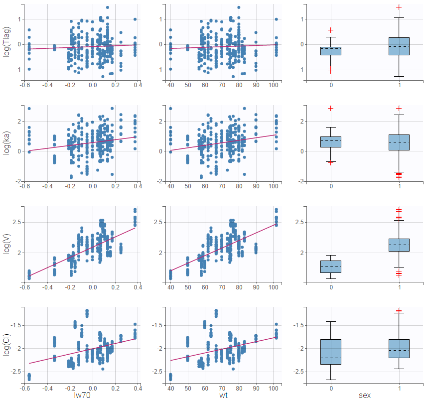
Visual guidelines
In order to help identifying correlations, regression lines, spline interpolations and Pearson correlation coefficients can be overlaid on the plots for continuous covariates. Here we can see a strong correlation between the parameter V and the covariate lw70.
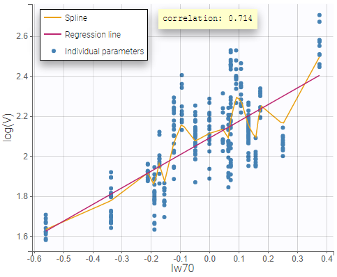
Highlight
Hovering on a point reveals the corresponding individual and, if multiple individual parameters have been simulated from the conditional distribution for each individual, highlights all the points points from the same individual. This is useful to identify possible outliers and subsequently check their behavior in the observed data.
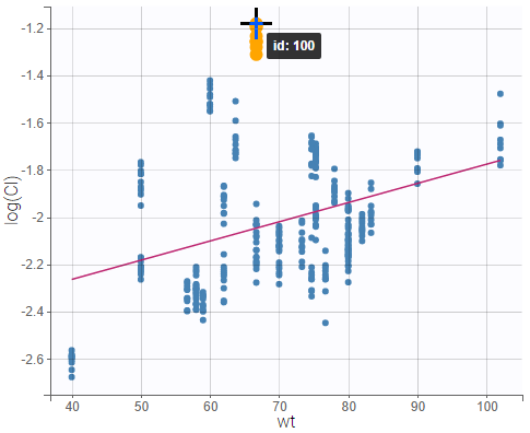
Selection
It is possible to select a subset of covariates or parameters, as shown below. In the selection panel, a set of contiguous rows can be selected with a single extended click, or a set of non-contiguous rows can be selected with several clicks while holding the Ctrl key. This is useful when there are many parameters or covariates. In particular, it is frequent to introduce transformed covariates, the selection allows to focus on the transformed versions rather than the original.
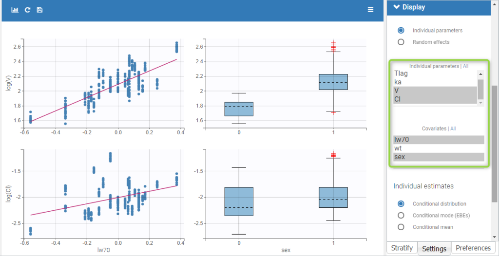
Comparing individual parameters and random effects
By default, the values on the Y-axis are computed with the individual parameters. One can choose to display the random effects instead. If some individual parameters are already modelled with covariates, this is taken into account by the random effects values, thus allowing to focus on remaining correlations.
The figures below show the diagnosis plots with individual parameters or random effects when the models for parameters V includes the covariate lw70. On the top, one can identify the correlations between individual parameters and covariates: the log-volume (log(V)) clearly increases with the log-transformed weight, as well with sex. On the other hand, the random effects on the bottom allow to focus on correlations that are not yet taken into account in the covariate model. Because the model already includes a linear relationship between the log-volume and the log-transformed weight, 
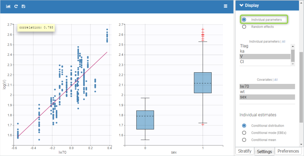
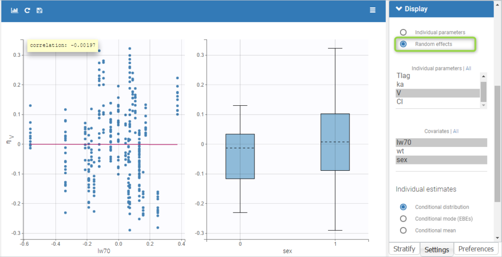
Stratification
Stratification can be applied by creating groups of covariate values. As can be seen below, these groups can then be split, colored or filtered, allowing to check the effect of the covariate on the correlation between two parameters. The correlation coefficient is updated according to the split or filtering.
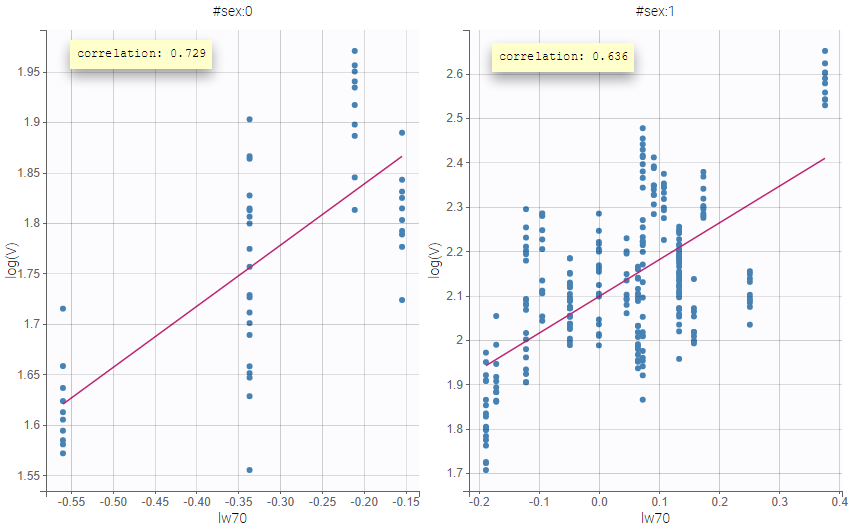
Settings
- General
- Legend and grid : add/remove the legend or the grid. There is only one legend for all plots.
- Correlation: display/hide the correlation coefficient associated with each scatter plot.
- Display
- Y-axis. The user can choose to see either the individual parameters or the random effects.
- Selection. The user can select some of the parameters or covariates to display only the corresponding plots. A simple click selects one parameter (or covariate), whereas multiple clicks while holding the Ctrl key selects a set of parameters.
- Individual estimates. The user can define which estimators are used for the definition of the individual parameters and thus for the random effects (conditional mean, conditional mode, simulated parameters)
- Visual cues. Add/remove a regression line or a spline interpolation.
By default, all plots are proposed with simulated individual parameters.
6.5.Predictive checks and predictions
6.5.1.Visual predictive checks
- Purpose
- Examples
- Details
- Settings
- Generating predictive checks on an external data set
- Exporting VPC simulations
- Correcting the VPC for missing observations
- Troubleshooting
Purpose
The VPC (Visual Predictive Check) offers an intuitive assessment of misspecification in structural, variability, and covariate models. The principle is to assess graphically whether simulations from a model of interest are able to reproduce both the central trend and variability in the observed data, when plotted versus an independent variable (typically time). It summarizes in the same graphic the structural and statistical models by computing several quantiles of the empirical distribution of the data after having regrouped them into bins over successive intervals.
More precisely, the goal is to compare the two following elements:
- Empirical percentiles: percentiles of the observed data, calculated either for each unique value of time, or pooled by adjacent time intervals (bins). By default, the 10th, 50th and 90th percentiles are displayed as green lines. These quantiles summarize the distribution of the observations.
- Theoretical percentiles: percentiles of simulated data are computed from multiple Monte Carlo simulations with the model of interest and the design structure of the original dataset (i.e., dosing, timing, and number of samples). For each simulation, the same percentiles are computed across the same bins as for empirical percentiles. Prediction intervals for each percentile are then estimated across all simulated data and displayed as colored areas (pink for the 50th percentile, blue for the 10th and 90th percentiles). By default, prediction intervals are computed with a level of 90%.
If the model is correct, the observed percentiles should be close to the predicted percentiles and remain within the corresponding prediction intervals.
Examples
VPCs vary slightly for different types of data. For joint models for multivariate outcomes, VPCs are available for each outcome.
- Continuous outcomes
warfarinPK_project (data = ‘warfarin_data.txt’, model = ‘lib:oral1_1cpt_TlagkaVCl.txt’)
In the following example, the parameters of a one-compartment model with delayed first-order absorption and linear elimination are estimated on the warfarin dataset. A constant residual error model was used. The figure presents the VPC with the prediction intervals for the 10th, 50th and 90th percentiles. Outliers are highlighted with red dots and areas. Here the three quantiles appear closer together than the model would suggest, therefore the VPC suggests that a proportional component should be added to the error model.
Since version 2024, there are options for displaying the x-axis using either nominal time, time after the last dose or regressors, if they are available in the dataset and appropriately tagged. You can choose these options within the x-axis settings of the plot settings.
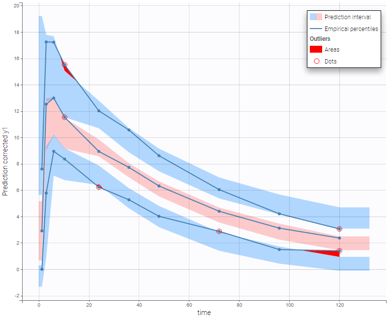
For joint models for continuous PK and time-to-event data, VPCs are available for each type of data. However it is important to note that dropout events are not taken into account in the VPC corresponding to the continuous data. Therefore, in the case of non-random dropout events in the dataset, this can result in discrepancies between observed and simulated data and thus hamper the diagnosis value of the VPC. Correcting this bias would require to include the simulated dropout in VPC, as well as adapt the design structure to compensate observed dropouts, an approach that is problematic when the design structure is complex. More details on this approach are given here.
- Non-continuous outcomes: count data and categorical data
VPCs for count data and categorical data compare the observed and predicted frequencies of the categorized data over time. The predicted frequency is associated with a blue prediction interval.
The following figure shows the VPC for a project with a continuous time Markov chain model and time varying transition rates.
- markov3b_project (data = ‘markov3b_data.txt’, model = ‘markov3b_model.txt’)
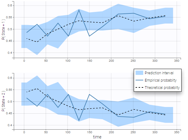
In addition to the categorization over time (binning on X), count data are also binned into groups of count values on the VPC (binning on Y). The number of bins and binning method can be set in Settings under “Y Bins”.
As an example, the VPC below corresponds to a project where a Poisson model is used for fitting the data. Observations are binned in 3 groups on the Y axis and 20 bins on the X axis.
- count1a_project (data = ‘count1_data.txt’, model = ‘count_library/poisson_mlxt.txt’)
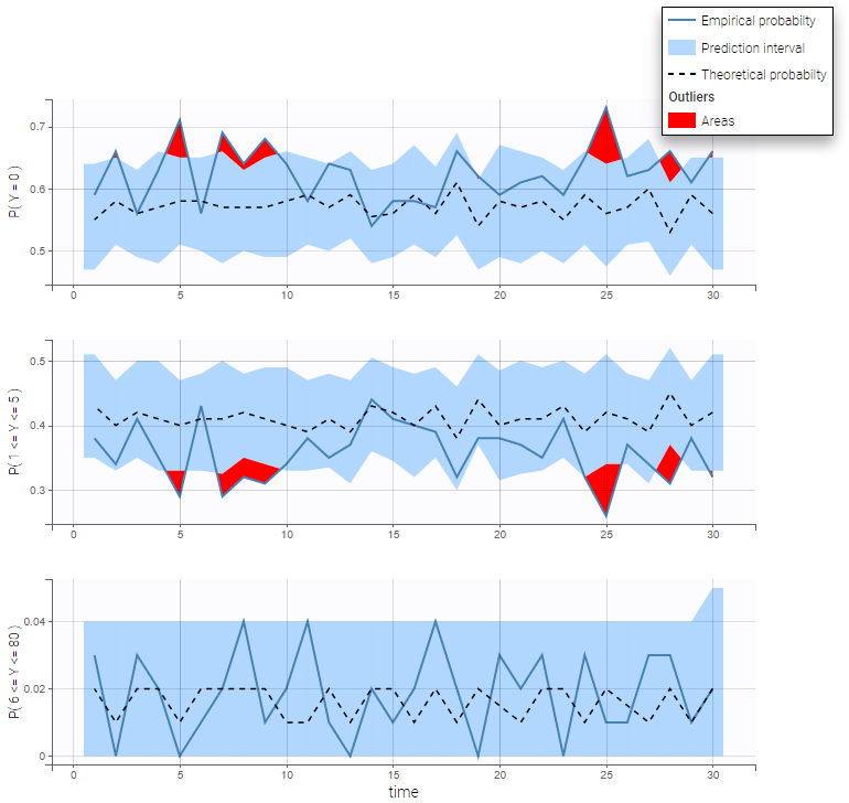
- Time-to-event data
In case of time-to-event data, two visual predictive checks are available, survival function based on the Kaplan-Meier plot for exactly observed events and the Turnbull estimator for the interval censored data, and the mean number of events per individual using Turnbull estimation (see here and here for reference papers).
Details on the VPC for TTE generation in Monolix are presented here.
The example below shows these two figures, computed with a model for the survival of patients with advanced lung cancer from the Veterans’ Administration Lung Cancer study. Censored data has been selected and displayed on the Kaplan-Meier plot. Note that censored data also cause an over prediction bias in the VPC based on the mean number of events per individual, because censored individuals contribute to the prediction interval but not to the empirical curve.
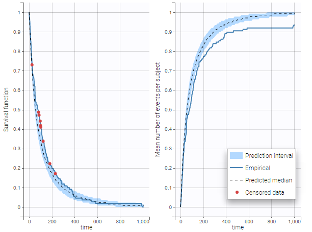
Sometimes numerical errors can appear in the simulations used for the TTE VPC. For example, when simulating a joint model with tumor growth and survival over a long time scale, the simulated hazard for death can become too high for some individuals at high times. In Monolix2021R1, the appearance of NaNs in the VPC simulations does not stop the generation of the VPC. The simulated individuals with NaNs in their simulations are not used in the prediction interval, and the percentage of simulated individuals with NaNs is then displayed in the Warnings.
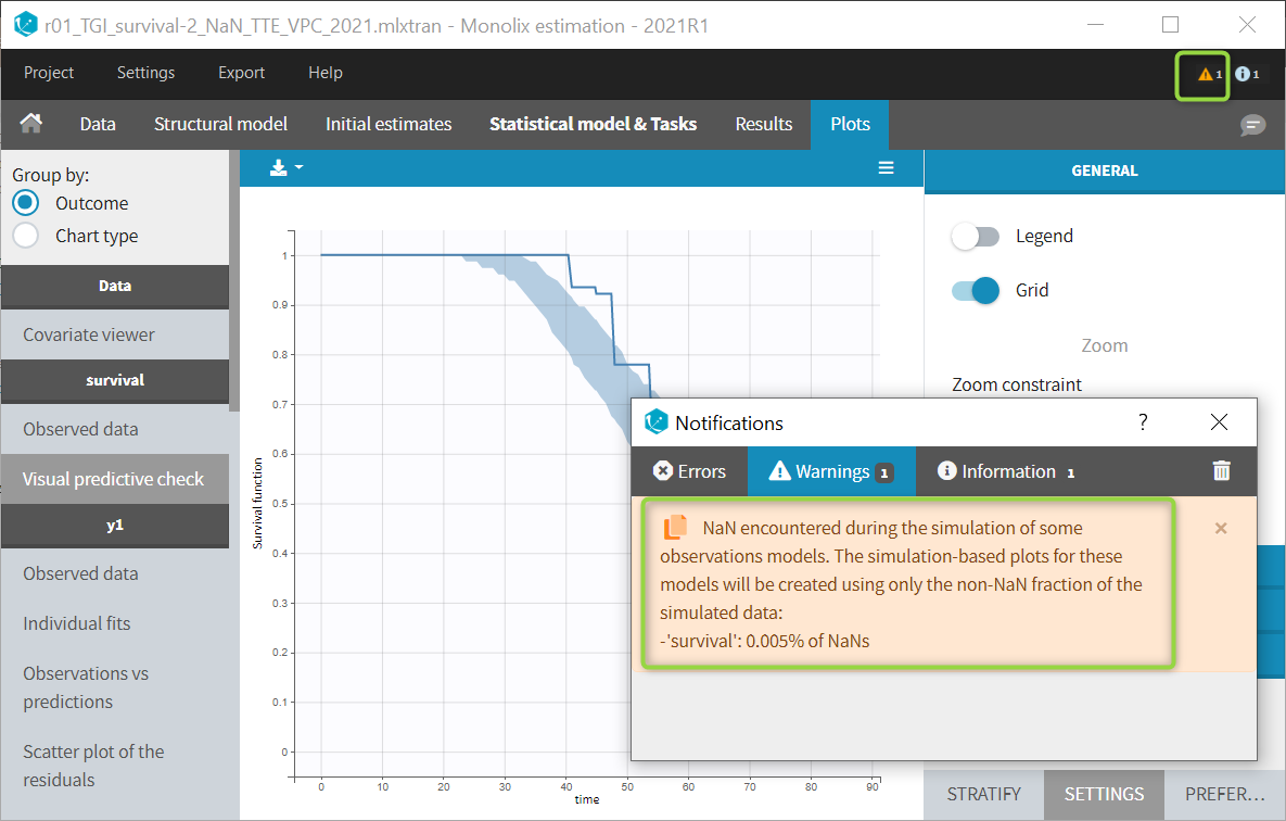
Details
- Binning criteria
Correctly defining the intervals (or bins) into which the data are grouped is crucial to construct a VPC that avoids distortion between the original and approximated distributions. Several strategies exist to segment the data: equal-width binning, equal-size binning, and a least-squares criterion. The number of bins can also be either set by the user, or automatically selected to obtain a good tradeoff. Indeed, a small number of bins leads to a poor approximation but a good estimation of the data’s distribution, while a large number of bins leads to a good approximation but poor estimation.
As an example, the VPCs below are computed on the PK model built for remifentanil pharmacokinetics, a dataset that involves a large variability in doses. The bins are delimited with vertical lines. The first VPC on the left is computed with 5 bins, the number automatically selected for this dataset. On the other hand, the second VPC on the right is computed with 15 bins. We notice that in this case the heterogeneity of the data results in a poor estimation of the data’s distribution. To keep a good estimation, a small number of bins is required, but the approximation then prevents from visualizing the kinetics in details. The absorption phase is for example not visible.
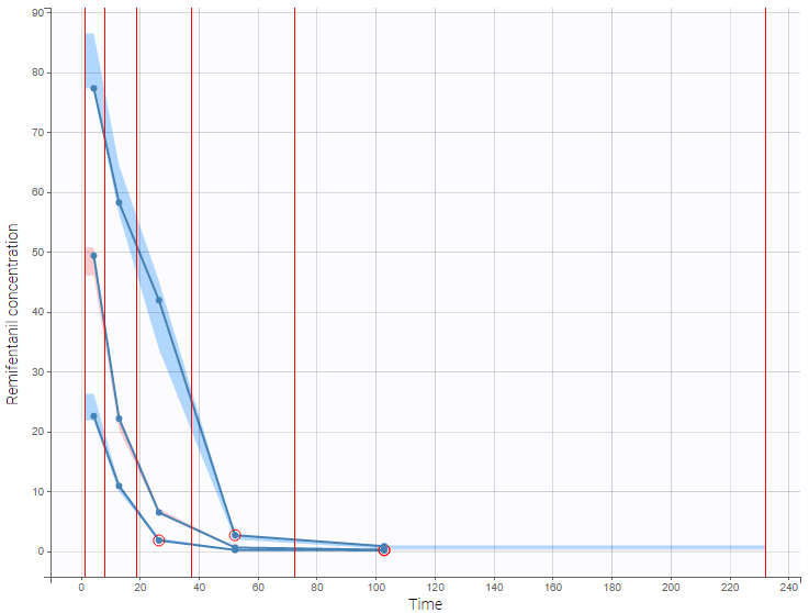
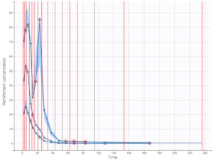
- Corrected predictions
As shown above, VPCs can be misleading if applied to data that include a large variability in dose and/or influential covariates, or that follow adaptive designs such as dose adjustments. The prediction-corrected VPC (pcVPC), with prediction correction, was developed to maintain the diagnosis value of a VPC in these cases. In each bin, the observed and simulated data are normalized based on the typical population prediction for the median time in the bin. Formulae are applied as in the publication from Bergstrand et al. In the simple case of normally distributed observations and a zero lower bound for observations, we get:
\[ pcY_{ij} = Y_{ij} \frac{\tilde{PRED}_{bin}}{PRED_{ij}} \]
where
- Yij : observation or prediction for the ith individual and jth time point,
- pcYij : prediction-corrected observation or prediction,
- PREDij: typical population prediction for the ith individual and jth time point
- PRẼDij: median of typical population predictions for the specific bin of independent variables.
This removes the variability coming from binning across independent variables.
The example below shows the pcVPC computed on the PK model built for remifentanil pharmacokinetics with 15 bins: the figure now gives a good estimation of the data’s distribution, including the absorption phase.
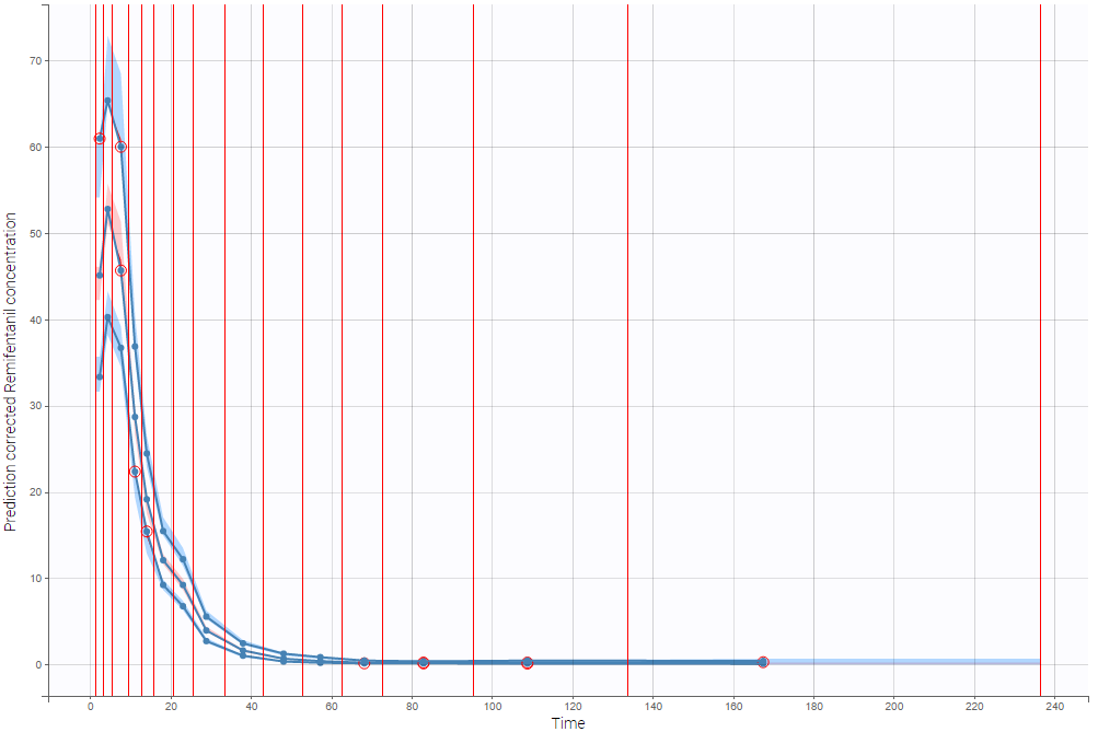
- Stratification
When possible, another useful approach to deal with heterogeneous data can be to split the VPC into groups of subjects that are more homogeneous. As an example, the VPCs below are computed again on the PK model built for remifentanil pharmacokinetics, with 15 bins, but the data was first split by a categorical covariate that characterizes groups of similar doses.
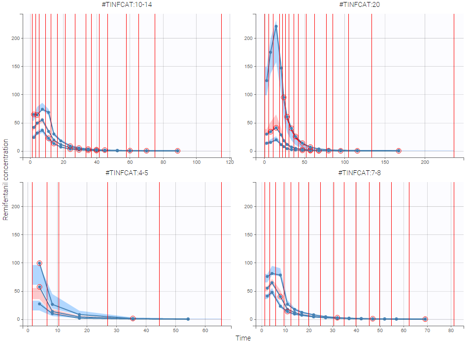
- VPC based on time after last dose (continuous data only)
Option in the display panel “Time after last dose” displays the VPC with data for times (the X-axis) after last dose (for Monolix versions 2021 and above). Below is an example with result for the demo project multidose_project.mlxtran (Monolix demo folder 6.3). Observed data overlaid the VPC. On the left image the X-axis is “Time”, and on the right the X-axis is “Time after last dose”. The exported charts data for the VPC include two columns for time and time after last dose – independently of the option selected in the interface. Doses with amount=0 are handled as the others. For observations before the first dose (or if no doses at all), time remains unchanged (i.e time after last dose = time). Finally, all administration ids are handled together (it is not possible to define time after dose for adm id = 2 only for instance).
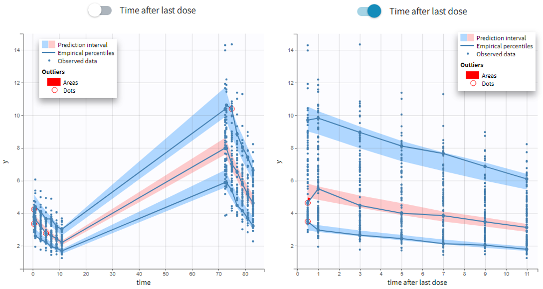
- Axis limits
From the 2023 version on, the user can choose the axis limits manually. This is particularly convenient when the prediction intervals go into negative values and log-scale is used on the y-axis. In that case, the VPC is shown by default from 1e-16 to the maximum value, which leads to an unreadable plot. After toggling the setting “custom limits” on, the axis limits can be selected by the user. As the other plot settings, the axis limits are copied to the placeholders when preparing a report.
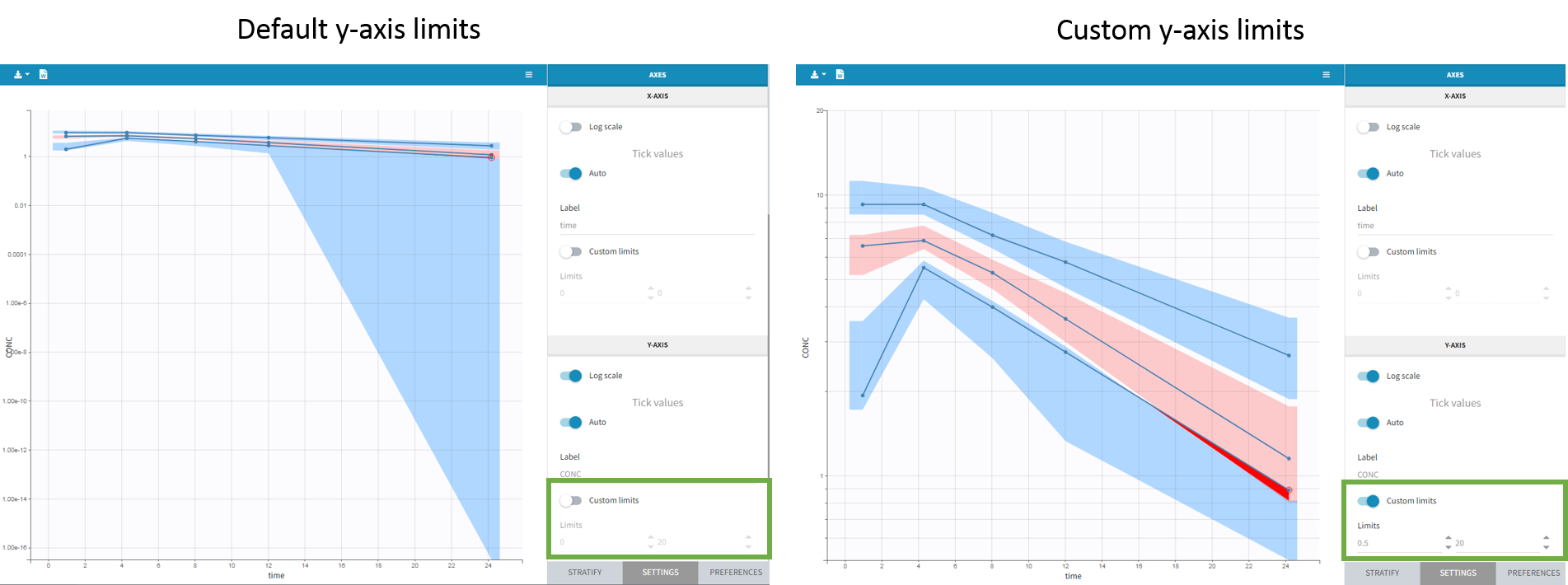
Settings
- General: Add/remove legend or grid
- Subplots (for TTE data)
- Add/remove plot for survival function (Kapan-Meier plot) or plot for mean number of events per individual
- Add/remove plot for survival function (Kapan-Meier plot) or plot for mean number of events per individual
- Display
- Observed data
- Observed data: Add/remove observed data.
- BLQ: Add/remove BLQ data if present.
- Use BLQ: Choose to use BLQ data or to ignore it to compute the VPC. BLQ data can be simulated, or can be equal to the limit of quantification (LOQ). The latter case induces strong bias .
- Empirical percentiles: Add/remove empirical percentiles for the 10%, 50% and 90% quantiles.
- Predicted percentiles: Add/remove theoretical percentiles for the 10% and 90% quantiles.
- Prediction interval: Add/remove prediction intervals given by the model for the 10% and 90% quantiles (in blue) and the 50% quantile (in pink).
- Set interpercentile level and higher percentile for prediction intervals (for continuous data by default the level is 90 and the higher percentile is 90%), or number of bands for TTE data
- Outliers
- Dots: Add/remove red dots indicating empirical percentiles that are outside prediction intervals
- Areas: Add/remove red areas indicating empirical percentiles that are outside prediction intervals
- Calculations
- Observed data
-
-
- Corrected predictions: compute the pcVPC using Uppsala prediction correction (see details above)
- Linear interpolation: Set piece wise display for prediction intervals (by default the display is linear)
- Time after last dose: Use time after last dose instead of time on the X-axis.
-
- Bins – for categorical data, X Bins and DV Bins (for Y axis) can be specified
- Bin limits: Add/remove vertical lines on the scatter plots to indicate the bins.
- Binning criteria: Choose the bining criteria among equal width (default), equal size or least-squares
- Number of bins: Choose a fixed number of bins or a range for automatic selection, and a range for the number of data points per bin.
- Axes
- Label: nore that “prediction corrected” and “after last dose” are added automatically when chooseing these settings and cannot be removed
- Log-scale
- Variable for x-axis: time, time after last dose (time relative to the previous dose), or regressor from the dataset
- Axis limits
All colors, points and lines can be modified by the user.
Generating predictive checks on an external data set
This video shows how to generate an external VPC in Monolix: a VPC that compares the simulations based on a population model estimated on a first data set to a second data set, for example to check whether a population model estimated on a single dose study is also valid on a new multiple dose study for the same molecule.
Exporting VPC simulations
When exporting the charts data, by default the charts data for the VPC include the observed data and predicted percentiles, but not the detailed simulations, which are usually quite large. Starting from the 2020 version, the user can nonetheless choose to include the VPC simulations by clicking on “Export > Export VPC simulations” in the application menu:
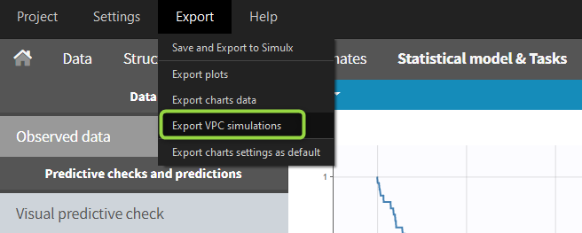
The simulated values are saved in <result folder>/ChartsData/VisualPredictiveCheck/XXX_simulations.txt. They can be used to replot the VPC in R for instance.
In Monolix2021 it is also possible to include systematically the VPC simulations in the exported charts data with an option in the Preferences: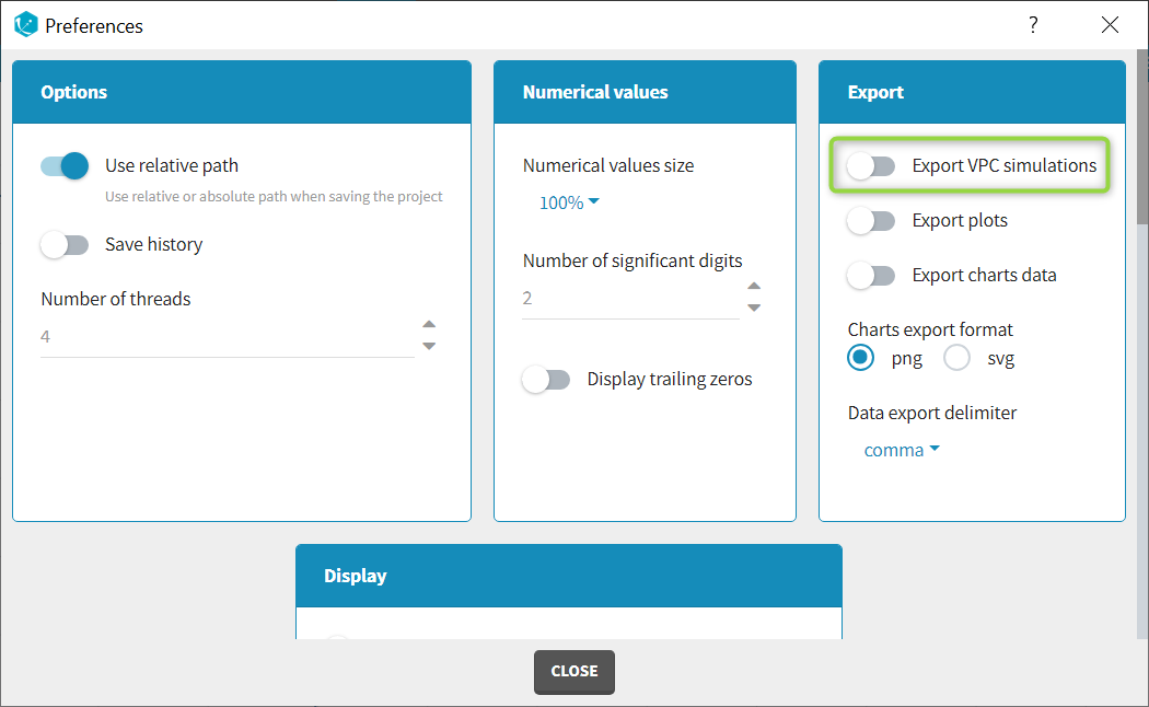
Correcting the VPC for missing observations
Missing observations can cause a bias in the VPC and hamper its diagnosis value. This page discusses why missing censored data or censored data replaced by the LOQ can cause a bias in the VPC, and how Monolix handles censored data to prevent this bias. It also explains the bias resulting from non-random dropout, and how this can be corrected with Simulx.
Troubleshooting
If the VPC plot is emtpy or with non-appropriate axis limits, follow the procedure below.
![]()
The problem appears after having clicked “Export > Export charts settings as default” on a previous project where the y-axis limits were different and this is now applied as default. It is possible to delete the default setting corresponding to the axis limits in the following way:
-
- Open the file C:/Users/<username>/lixoft/monolix/monolix2023R1/config/settings.default in a text editor
- Delete the following lines:
VPCContinuous\yInterval= ...
outputPlot\yInterval= ...
- Save the file
- Reopen your project
6.5.1.1.VPC for Time-To-Event data
The construction of a VPC plot for time-to-event data in Monolix requires several steps:
- 1. Simulation of datasets. First, Monolix simulates datasets using the population model, which contains the structural and statistical models and the estimated population parameters.
- 2. Survival function estimators. Then, for the original dataset and each simulated dataset, it estimates the survival function with either the Kaplan-Meier estimator for exactly observed events or the Turnbull estimator for interval censored events.
- 3. Prediction interval. Finally, Monolix calculates lower and upper percentiles of the simulated survival function estimates, which give a prediction interval.
1. Simulation of TTE data sets using a population model
Simulations of time-to-event datasets give, for each individual, times when an event occurs. The simulations are based on the same design as in the original data set, the same number of individuals as in the original data set and individual parameters are sampled using the covariates from this original data set and the population parameters estimated in Monolix.
To simulate a time when an event occurs, (u) is defined as a probability that an event (X) occurs before a certain time (T). This probability is computed using the cumulative hazard function (H(t))
 = 1-exp\left(-\int_0^T h(t,\psi_i) dt\right) = 1-exp(-H(T)),")
where \(H\) is a solution to the ODE system \(dH/dt = h\). A value of the probability \(u\) is sampled from the uniform \([0,1]\) distribution, thus in the above equation the time T becomes the unknown variable. A root finding method from an ODE solver finds its value.
The time T is not a given independent variable, but it is a simulated observation. Moreover, simulations are only until the time \(T_{max}\), which corresponds to the last time found in the data set. This value is the final integration time of the ODEs for each individual and it also defines a unique right censoring time for all individuals in the simulated data sets. It is independent of the individual times of events or right censoring in the original data set.
If the simulation fails because of a numerical error (e. g. because of a too high hazard), the simulated individuals with NaNs in their simulations are not used in the prediction interval, and the proportion of simulated individuals involved is then displayed in the interface.
Example
In this example, the individual 3 in the original data set (table on the left) experienced an event at time 4. In the simulations (tables on the right), an event for this individual can occur before or after that time, or may occur after \(T_{max}=5\) (last table). Similarly, while the individual 5 left the study at time 3 without experiencing an event in the original data set, in the simulations for this individual an event can occur before or after time 3. If an event has not occurred at \(T_{max}=5\), then it is right censored.
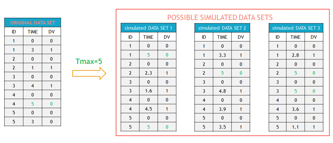
Possible sources of bias in the simulations
Censoring (dropout)
In the original dataset (input Monolix dataset), censoring can be at any time: because the patient drops out or because the study is stopped for instance. In contrast, simulated datasets have no dropout until the global Tmax over all individuals, which means that there are on average more events in the simulated datasets than in the original dataset. However, if censoring in the original dataset is truly random, simulating until the global Tmax over all individuals should not produce a bias because the “additional” simulated events are evenly distributed over time. But if censoring in the dataset is not truly random, the empirical Kaplan-Meier curve is biased while the VPC predictions are not, so it may appear as a misfit. If we would instead censor the simulated datasets at the same censoring times as in the original dataset (Tmax=5 for id 4 and Tmax=3 for ID 5 on the above example), this could introduce other bias.
Regressor
If the TTE model depends on a regressor, the regressor is interpolated using last value carried forward.
Doses
If the TTE model depends on a PK model with doses present in the dataset, it is important to also include the planned (but not given because of event or dropout) doses in the dataset such that the doses span the same time range for all individuals. Otherwise this will create a bias in the VPC.
2. Survival function estimators
Given some survival data that includes censoring (right-censoring or interval-censoring), a survival function can be estimated as a non-parametric maximum likelihood estimator (NPMLE).
Thus Monolix estimates an NPMLE for each simulated dataset, depending on the event type:
- Kaplan-Meier estimator for exactly observed events.
- Turnbull estimator for interval censored data.
The calculation of these estimators is detailed in the next sections.
Note: for interval censored data, the Turnbull estimator is used only in the VPC:
- In the plot of Observed data, Monolix assumes that all events are exactly observed and displays the data using the Kaplan-Meier estimator explained in the previous section. This is because that plot is generated right after accepting the dataset, before a model has been selected. However, just looking at the dataset, the case of exact and interval censored events are indistinguishable. For example: assume that an observation period started at \(t=0\) and at \(t=1\) an event is marked by 1 in the column for the observation. Without any other information, the event could have occurred at \(t=1\) or before.
- In the VPC, Monolix uses the eventType information specified in the structural model. If “eventType = intervalCensored” is specified in the structural model, Monolix uses the Turnbull estimator for empirical and simulated survival curves in the VPC, in order to avoid bias in the survival function estimate. If eventType is not specified in the structural model, Monolix considers all interval-censored events as exactly observed at the end of a censored interval, and uses the Kaplan-Meier estimator.
DEFINITION:
Event = {type = event, eventType = intervalCensored, intervalLength = L,
                maxEventNumber = 1, hazard = h}
2.1. Exact events: Kaplan-Meier estimator
The Kaplan-Meier estimator, or product limit estimator, is a type of non-parametric maximum likelihood estimator and a standard method to approximate the survival function \( S(t) \) in the case of exact events. It describes the probability that an individual survives until time t, knowing that it survived at any earlier time. For single events, it is given by the following formula:
=\prod_{i:t_i<t} \left(1-\frac{d_i}{n_i}\right),")
where
- \(t_i\) – times before t, when at least one event occurred,
- \(d_i\) – number of events at the time \(t_i\),
- \(n_i\) – number of individuals at risk, that is who did not experience an event until \(t_i\).
The probability \((p_e)\) of an event is the ratio between the number of occurred events \((d_i)\) and the number of individuals at risk \((n_i)\). The complement of it, \((1-p_e)\), gives an estimation of the survival. For each time t, the total number of individuals at risk, who survived, may change. Thus, the current survival probability is the product of all probabilities at previous times \(t_i\), when at least one event occurred.
This formula can be better understood by calculating for example the probability that a patient survives 2 days: it is a product of two probabilities: the probability that the patient survives the first day and a conditional probability that they survive the second day, knowing that they survived the first one.
Example:
On the left of the figure below, a typical example of a time-to-event data set contains information about exact times when individuals experienced an event (T=1) or when they left the study (drop-out: T=0). Five individuals have two observations each: the time at which the observation starts (T=0 for everyone) and the time of an event. If a patient leaves the study, then the dataset contains a drop-out time with T=0, instead of T=1, in the column for the observations. This means that the patient experienced no event but survived until the drop-out time. The Kaplan-Meier estimator takes into account such situations, because these individuals are not counted as individuals at risk (they are not counted in the denominator \(n_i\)) at later times.
The study starts at time \(t_1\). There are no events, so \(d_1=0\) and the value of the Kaplan-Meier estimator is 1. Until the next event time at \(t_2=1\), the estimator remains constant. At that time, one individual experienced an event, hence \(d_2=1\), and all individuals survived until that time so \(n_2=5\). As a result, the probability to survive decreases by 0.2. It is the height of the jump at \(t=1\) in the plot. The Kaplan-Meier estimator remains constant until the next event. At time \(t=3\) there are two events. The number \(n_3\) counts now only 4 individuals – it has decreased by 1 due to the previous event. The final probability at time 3 is a product of all earlier probabilities. At \(t=4\) there is a drop-out: patient 5 left the study without experiencing an event. The survival curve remains constant and a red dot marks the drop-out. The Kaplan-Meier estimator takes into account this situations, because at the next event time \(t=5\), this individual is not counted as an individual at risk – thus the denominator n will be smaller. Finally, at time \(t=5\), there is only one individual left, and one event, so the survival becomes 0.
Remarks
- The Kaplan-Meier estimator handles correctly the information about individuals who left the study (right-censoring), but there is a bias when the exact times of events are unknown (interval-censoring).
- In the TTE VPC, Monolix estimates a linear approximation of the Kaplan-Meier estimate.
2.2 Interval censored events: Turnbull estimator
The Turnbull estimator is a generalization of the Kaplan-Meier estimator that allows for interval censoring. In the TTE VPC, Monolix uses this estimator to plot both the empirical and simulated survival curves.
Interval censored events do not occur at exact times \( t_i \), \(i = (1,…,n) \), but within some time intervals between times \( L_i \) and \( U_i \), \( L_i < t_i \leq U_i \). In case of right censored data (dropout), \( L_i\) is the time when the individual leaves the study, and \( U_i = +\infty \): an event will occur within the interval \( (L_i, +\infty) \).
In the TTE VPC, the intervals \( (L_i, U_i] \) are:
-
- For the empirical survival curve, they correspond to the censoring intervals of the original data set.
- For simulated survival curves, the definition of these intervals depends on whether the structural model contains the option “intervalLength” or not:
- If “intervalLength=L” is given, then the intervals are \([0, L], (L, 2\cdot L],\dots , (m\cdot L,T_{max} ]\)
- If “intervalLength” is missing, then the whole period of observation defined with the minimal and maximal times in the data is split in 10 regular intervals.
Note: Simulations of interval censored datasets give, as in the case of exactly observed events, exact times of events for each individual. In order to compare the simulated survival to the empirical survival without bias, simulated events are counted in regular intervals to be transformed into interval censored events, and they are then represented in the VPC with the Turnbull estimator just like for the empirical survival.
Turnbull intervals
The Turnbull estimator is computed on time intervals \( (\tau_{j-1} , \tau_j] \) that are called Turnbull intervals:

This grid of times is constructed from all points \( L_i, U_i \) for \( i = 1,…,n\) in increasing order.
Turnbull algorithm
Notations
- The probability that an event occurs in a j-th Turnbull interval is
- For each individual \( i\): \( \alpha_i \) denotes a weight such that
The Weight \(\alpha_{ij} \) is an event indicator – it indicates whether an event from the interval \( (L_i, U_i] \) occurred at \( \tau_j \).
- \(d_j\) is the number of events until \(\tau_j\) and \(n_j\) is the number of individuals at risk at \(\tau_j\)
- The likelihood function for \(p = (p_1, …, p_{m+1})\) is:
 = S(\tau_{j-1}) - S(\tau_j)")
![\alpha_i = 1\cdot { (\tau_{j-1} , \tau_j] \subset (L_i, U_i] }.](http://s0.wp.com/latex.php?latex=+%5Calpha_i+%3D+1%5Ccdot+%7B+%28%5Ctau_%7Bj-1%7D+%2C+%5Ctau_j%5D+%5Csubset+%28L_i%2C+U_i%5D+%7D.&bg=ffffff&fg=000&s=0 "\alpha_i = 1\cdot { (\tau_{j-1} , \tau_j] \subset (L_i, U_i] }.") The Weight \(\alpha_{ij} \) is an event indicator – it indicates whether an event from the interval \( (L_i, U_i] \) occurred at \( \tau_j \).
The Weight \(\alpha_{ij} \) is an event indicator – it indicates whether an event from the interval \( (L_i, U_i] \) occurred at \( \tau_j \).![L_S(p)= \prod_{i-1}^n [S(L_i) - S(R_i)] = \prod_{i-1}^n\sum_{j=1}^{m+1}\alpha_{ij} p_j](http://s0.wp.com/latex.php?latex=L_S%28p%29%3D+%5Cprod_%7Bi-1%7D%5En+%5BS%28L_i%29+-+S%28R_i%29%5D+%3D+%5Cprod_%7Bi-1%7D%5En%5Csum_%7Bj%3D1%7D%5E%7Bm%2B1%7D%5Calpha_%7Bij%7D+p_j&bg=ffffff&fg=000&s=0 "L_S(p)= \prod_{i-1}^n [S(L_i) - S(R_i)] = \prod_{i-1}^n\sum_{j=1}^{m+1}\alpha_{ij} p_j")
Main idea of the Turnbull algorithm
Finding the NPMLE of S, denoted by \(\hat{S}\), means maximizing \(L_S(p)\) under the constraint that \(p_j\) are positive and \(\sum_{j=1}^{m+1} p_j = 1\). The original Turnbull algorithm (1976) is the first and the simplest method to maximize \(L_S(p)\) with respect to \(p\). It is an application of the Expectation-Maximisation (EM) algorithm.
Remark: \(L_S\) depends only on values of S at points \(\tau_j\), and the behaviour of S within the Turnbull intervals is unknown. The convention applied here is: \(\hat{S}(t) = \hat{S}(\tau_j)\) when \(\tau_{j-1}\leq t\leq \tau_j\).
Procedure
The algorithm is the following:
- Step 0: Initialization – choose an initial guess for \( S^{old}(\tau_j) \). This initial guess for S is the estimate obtained from the Kaplan-Meier estimator under the assumption that events occur at \( U_i \), interpolated on the \( \tau – \) grid.
- Step 1: Compute the probability of an event at time \( \tau_j \) as
 - S^{old}(\tau_j), j = 1,\dots ,m")
- Step 2: Estimate the number of events at \( \tau_j \) as

- Step 3: Compute the estimated number of individuals at risk at time \( \tau_j \)

- Step 4: Compute \(S^{new} \) using the Kaplan-Meier estimator using \( \tilde(d) \) and \( \tilde(n) \) to update the survival function
- Stopping criterion: If the updated solution \(S^{new} \) is close to the old solution \(S^{old} \) (in Monolix, \(\Vert S^{new} – S^{old} \Vert < 0.001\) ), stop, otherwise set \(S^{old} = S^{new} \) and repeat steps 1 – 4
Linear approximation
In the TTE VPC, just like for the the Kaplan-Meier estimate, Monolix calculates a linear approximation of the Turnbull estimate.
Example
Below we show a small dataset with interval censored events. The individuals are in increasing order of the times at which censored intervals end. The figure on the rights shows two curves:
- The upper bound curve is the Kaplan-Meier estimate assuming that events occur exactly at the upper interval limit \( t_i = U_i \).
- The lower bound curve is the Kaplan-Meier estimate assuming that events occur exactly at the lower interval limit \( t_i = L_i \).

For comparison, we show now a similar dataset corresponding to exactly observed events at the upper interval limit. The figure on the right shows again the Kaplan-Meier estimator, and in addition its linear approximation.
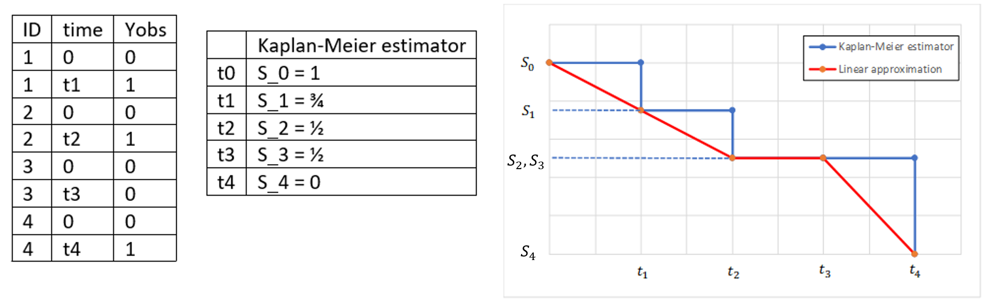
Procedure
The time points of the lower and upper interval limits for all individuals are ordered in increasing sequence. In this example, the assumption is


The Turnbull intervals are the intervals \( (\tau_{j-1},\tau_j]\), where \(j=1,\dots , m\), with \(\tau_0=0\) and \(\tau_8=\infty\).
The weights \( \alpha_{ij} \) are elements of the following matrix:
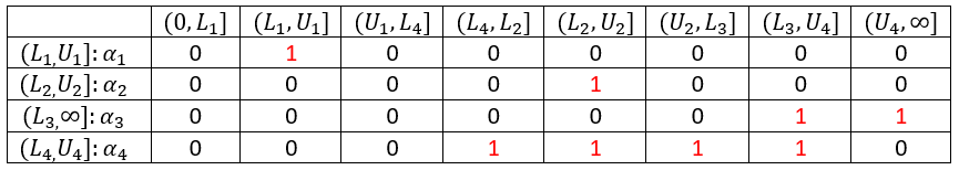
First iteration of the algorithm
Step 0: The initial guess is the upper bound curve, that is the Kaplan-Meier estimator under the assumption that events occur at \( U_i \), interpolated on the \( \tau – \) grid.
=1,\quad S^{old}(\tau_1)=1,\quad S^{old}(\tau_2)=S_1,\quad S^{old}(\tau_3)=S_1,\quad S^{old}(\tau_4)=S_1\newline S^{old}(\tau_5)=S_2,\quad S^{old}(\tau_6)=S_2,\quad S^{old}(\tau_7)=S_4,\quad S^{old}(\tau_8)=S_4")
Step 1: The probabilities that events occur in the Turnbull intervals are

Step 2: Modified number of events
\(\quad\quad\quad \tilde{d}_1=0\\
\quad\quad\quad\tilde{d}_2=\frac{\alpha_{12} p_2}{\alpha_{12} p_2 }=1\\
\quad\quad\quad\tilde{d}_3=0\\
\quad\quad\quad\tilde{d}_4=0\\
\quad\quad\quad\tilde{d}_5=\frac{\alpha_{25} p_5}{\alpha_{25} p_5 } + \frac{\alpha_{45} p_5}{\alpha_{45} p_5+\alpha_{47} p_7 }=1+\frac{S_1-S_2}{S_1-S_4 }\\
\quad\quad\quad\tilde{d}_6=0\\
\quad\quad\quad\tilde{d}_7=\frac{\alpha_{37} p_7}{\alpha_{37} p_7 } + \frac{\alpha_{47} p_7}{\alpha_{45} p_5+\alpha_{47} p_7 } =1+\frac{S_2-S_4}{S_1-S_4 }\\
\quad\quad\quad\tilde{d}_8=0\)
Step 3: Modified number of individuals at risk
\(\quad\quad\quad\tilde{n}_1=4\\
\quad\quad\quad\tilde{n}_2=4\\
\quad\quad\quad\tilde{n}_3=3\\
\quad\quad\quad\tilde{n}_4=3\\
\quad\quad\quad\tilde{n}_5=3 \\
\quad\quad\quad\tilde{n}_6=1+\frac{S_2-S_4}{S_1-S_4}\\
\quad\quad\quad\tilde{n}_7=1+\frac{S_2-S_4}{S_1-S_4}\\
\quad\quad\quad\tilde{n}_8=0\)
Step 4: Kaplan-Meier estimator for the modified values of \(d\) and \(n\):
\(\quad\quad\quad S^{new}(\tau_0)=1\\
\quad\quad\quad S^{new}(\tau_1) = 1\cdot (1-\frac{0}{4})=1\\
\quad\quad\quad S^{new}(\tau_2) = 1\cdot (1-\frac{1}{4})=\frac{3}{4}\\
\quad\quad\quad S^{new}(\tau_3) = \frac{3}{4}\cdot (1-\frac{0}{3}) = \frac{3}{4}\\
\quad\quad\quad S^{new}(\tau_4) = \frac{3}{4}\cdot (1-\frac{0}{3}) = \frac{3}{4}\\
\quad\quad\quad S^{new}(\tau_5) = \frac{3}{4}\cdot (1-\frac{1+\frac{1}{3}}{3}) = \frac{5}{12}\\
\quad\quad\quad S^{new}(\tau_6) = \frac{5}{12}\cdot (1-\frac{0}{1+\frac{2}{3}}) = \frac{5}{12}\\
\quad\quad\quad S^{new}(\tau_7) = \frac{5}{12}\cdot (1-\frac{1+\frac{2}{3}}{1+\frac{2}{3}}) = 0\\
\quad\quad\quad S^{new}(\tau_8) = 0\)
The figure below compares the linear approximations of Turnbull estimate at the start of the first iteration (\(S^{old}\)) and at the end (\(S^{new}\)), as well as the linear approximation of the Kaplan-Meier estimate in case of exact events.
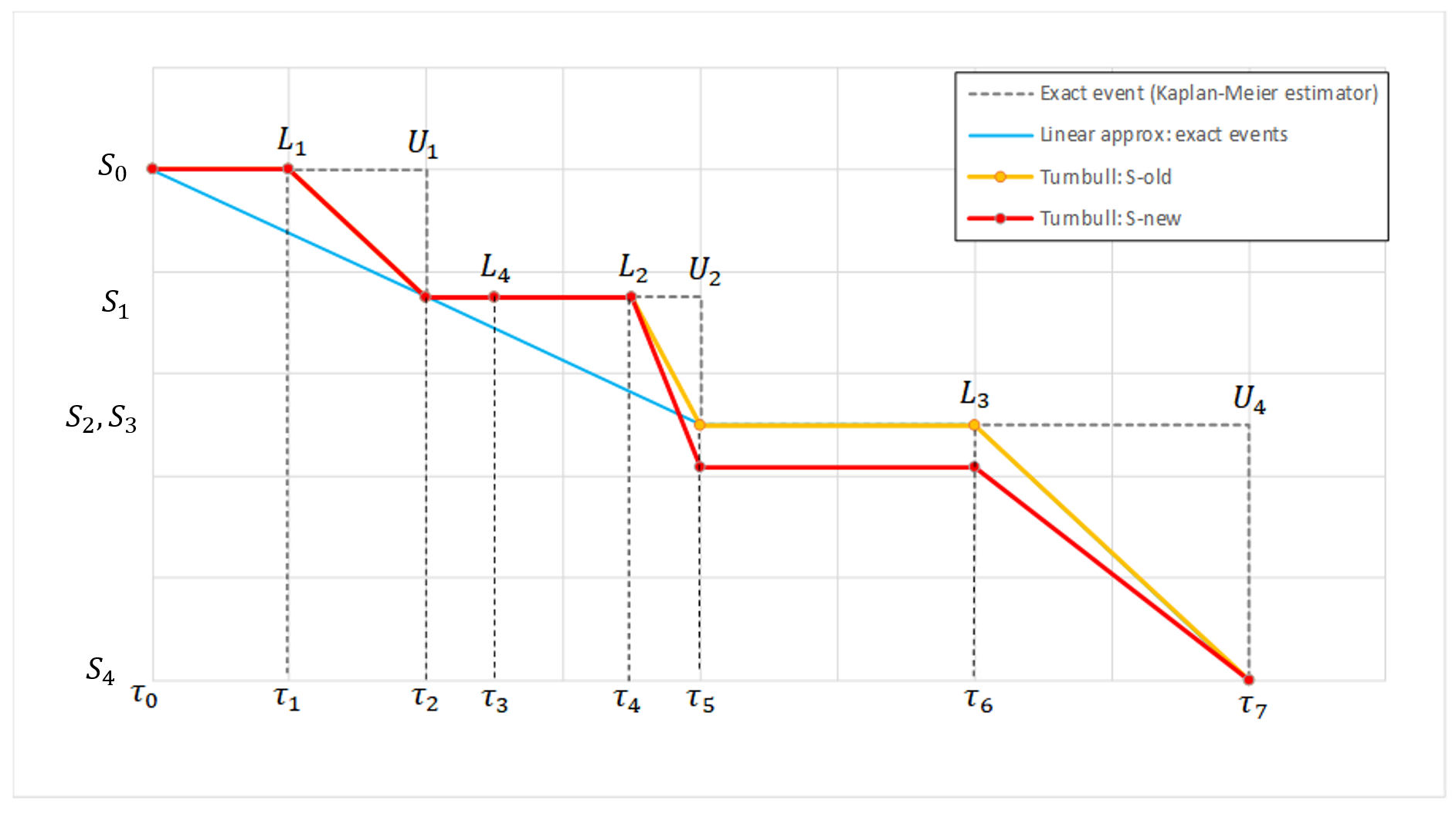
- The difference between the blue curve and \(S^{old}\) comes from the fact that \(S^{old}\) is interpolated on a grid including the \(L_i\) time points while they are not included in the grid considered in the case of exact events.
- The first iteration of the Turnbull agorithm has the effect of lowering \(S^{new} \)compared to \(S^{old}\) after \(\tau_4\), which is due to the fact that the event in \((L_4,U_4]\) may have already occured after that point.
3. Prediction interval
To generate the prediction interval in the VPC plot, Monolix performs by default 500 simulations with N individuals as in the original data set. As a result, it produces 500 time series that form 500 survival curves (based on Kaplan-Meier or Turnbull estimators). Since simulated event times are random numbers, all estimated survival functions have different time grids.This is shown on Fig.(a) with two different simulated datasets.
The interpolation of these curves on a fixed time grid allows to calculate the prediction interval. In Monolix the default time grid consists of a uniform grid with 100 points. For exactly observed events, the grid includes in addition all time points from the original data set to provide all possible information. Exact event times are unknown for interval censored events, so dataset time points have no additional information. This is shown on Fig.(b) with the Kaplan-Meier plot from the simulated dataset 1 from Fig.(a), interpolated on a different time grid than its events, combining regularly spaced points at times 0, 10, 20, …, 100, and additional time points indicated in green that come from the original dataset.).
The interpolation on the new grid gives at each time point of the grid a set of probabilities corresponding to different simulated survival curves. It allows to calculate lower and upper percentiles (the 5th and 95 percentiles are the default choice) and draw the prediction interval. This is shown on Fig.(c) with the survival estimators from multiple simulations on the same time grid as on Fig. (b).
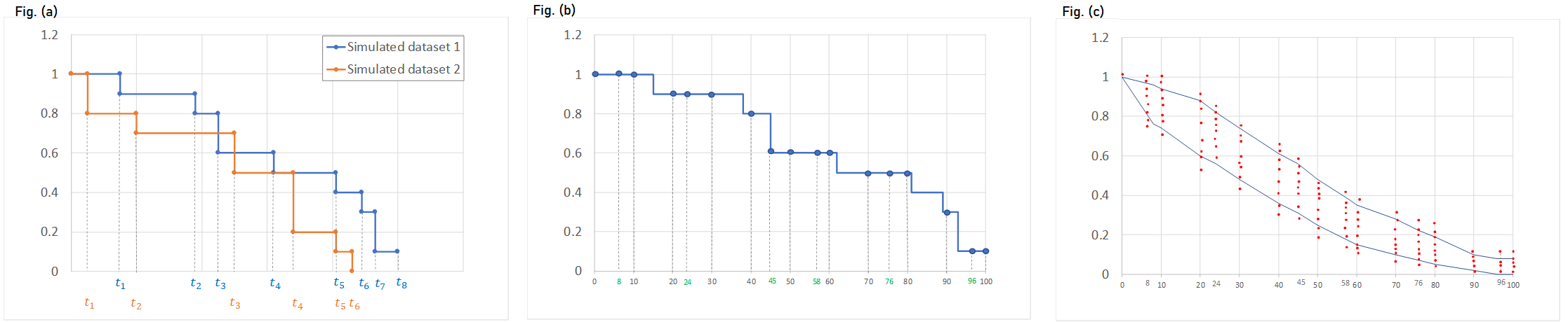
Example 1: exactly observed events
The dataset contains times of exactly observed single events of 30 individuals. The survival model has a constant hazard function and the Kaplan-Meier estimator approximates the survival function. The VPC plot uses a linear approximation of the Kaplan-Meier curve (Fig. on the left). By default, the fixed grid has 100 uniformly distributed points together with all time points from the date set. The figure on the left presents the VPC plot with the default settings. The approximation of the empirical and simulated Kaplan-Meier curves is sufficient on the default grid. In contrast, the VPC on the Figure on the right uses a grid with only time points from the original dataset. The accuracy of the prediction interval is decreased.
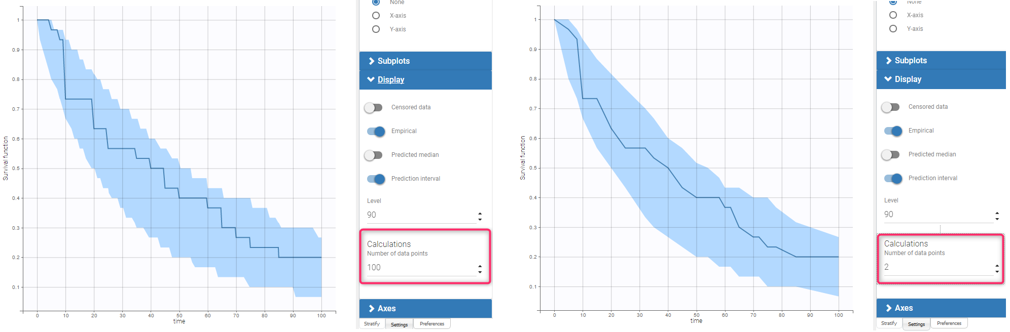
Example 2: interval censored events
In this dataset, the times of events from the previous example are the ends of time intervals within which events occurred. The length of the censored intervals in the dataset is non constant among individuals, and oscillates around 5. The structural model includes this information in eventTime and intervalLength options.
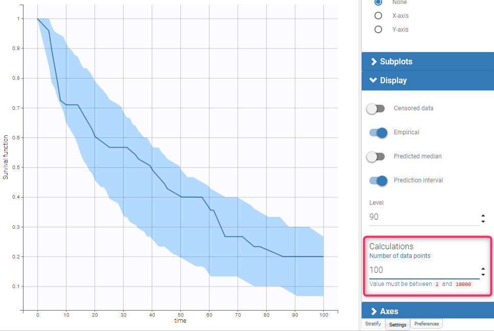
6.5.1.2.Correcting the VPC for missing observations
Missing observations can cause a bias in the VPC and hamper its diagnosis value. This mini case-study shows why missing censored data or censored data replaced by the LOQ can cause a bias in the VPC, and how Monolix handles censored data to prevent this bias. It also explains the bias resulting from non-random dropout, and how this can be corrected with Simulx.
Censored data and VPC
This section explains the different cases that can occur when some data are censored. If the censored data are marked in the dataset, they are handled by Monolix in a way that prevents bias in the diagnostic plots such as the VPC. The bias remains however if the censored data are missing.
Censored data missing from the dataset
The figures below show what happens if censored data are missing from the dataset. The figures on the left and middle focus on two individuals in a PK dataset, with their observed concentrations (on the left) or predicted concentrations (in the middle) over time as blue dots, and with similar measurement times. We assume that a good model has been estimated on this data. Three simulated replicates are represented on the same plot in the middle, although percentiles are calculated on each replicate separately in order to generate the prediction intervals on the VPC.
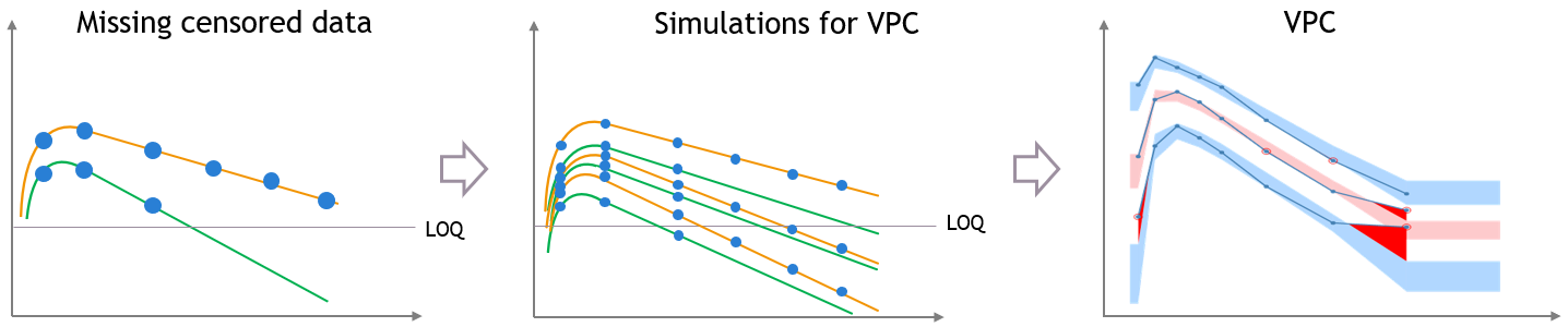
In case of missing censored data, the empirical percentiles represented by the blue lines on the VPC do not decrease much at high times, because only the individuals with high enough observations (like the orange individual, and not like the green individual) contribute to the percentiles.
The simulations for the VPC follow the same measurement times as the initial dataset, however if the variability is unexplained the predictions for all the individuals have the same prediction distributions, so the number of predicted observations that contribute to the prediction intervals are the same for each percentile. This results in a discrepancy between observed and simulated data, that can be seen in red.
Explained inter-individual variability
This bias is reduced if most of the variability in the predictions is explained by some covariate effects in the model. In that case the variability of the predicted concentrations at high times will match the variability in the measurement times, and the discrepancy is reduced and can diseappear. The diagnosis value of the VPC is improved, although the shape of the percentiles in the VPC is still affected by missing observations.
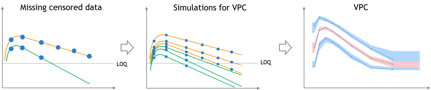
Censored data in dataset and “Use censored data” is OFF
If there is censored data in the dataset and the toggle “use censored data” in VPC plot display settings is off, the VPC is simulated for all times including censored times, and all values below the maximum LLOQ value and above the minimum ULOQ in dataset are dropped to calculate the percentiles.
The empirical percentiles are calculated using the non-censored times only.
“Use censored data” is ON and LOQ is used for calculations
In this case, the VPC is simulated for all times including censored times, and all simulated values are used to calculate the simulated percentiles.
For the empirical percentiles, the LOQ value in the dataset is used to replace the censored observations in the percentile calculation.
A strong bias appears in the VPC. The bias affects the empirical percentiles, as seen below, because the censored observations should actually be lower than the LOQ.
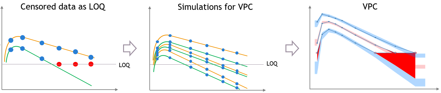
“Use censored data” is ON and simulated observations are used for calculations
In this case, the VPC is simulated for all times including censored times, and all simulated values are used to calculate the simulated percentiles.
For the empirical percentiles, the bias shown above is prevented by replacing the censored observations in the diagnostic plots by samples from the conditional distribution \(p(y^{BLQ} | y^{non BLQ}, \hat{\psi}, \hat{\theta})\), where \(\hat{\theta}\) and \(\hat{\psi}\) are the estimated population and individual parameters.
This corrects the shape of the empirical percentiles in the VPC, as seen on the figure below. More information on handling censored data in Monolix is available here.
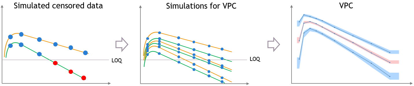
Dropout and VPC
The same kind of bias can also occur when the dataset is affected by non-random dropout events. In this section we take an example of tumor growth data. We assume that the data have been fitted with a good model, and is affected by non-random dropout, because individuals with a high tumor size quit the study or die. This means that no more observation for the tumor size is available after the time of dropout, represented with the dashed vertical lines.
A bias appears in the VPC, caused by the missing censored observations. This is because there are more missing observations in the dataset for high tumor sizes, which is not the case in simulated predictions from the model, unless the inter-individual variability is well explained by some covariate effects.
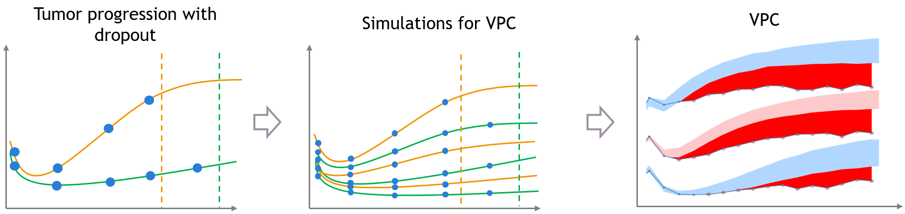
Correcting the bias from dropout
Correcting this bias requires to provide additional measurement times after the dropouts, which cannot be done automatically in Monolix without making strong assumptions on the design of the dataset. However, it can be attempted with simulations in Simulx, with additional measurement times chosen by the user in adequation with the dataset, and some post-processing in R.
The correction also requires to model the dropout with a time-to-event model, that should depend on the tumour size. After estimating the joint tumor growth and time-to-event model in Monolix, it becomes possible to predict the time of dropout for each individual. The predictions for dropout times we will use for post-processing in R.
The figure below shows the main steps for correcting the bias from dropout in a VPC. The VPC (on the bottom of the figure) can be regenerated with new simulations in Simulx (shown on the top of the figure) and with some plotting functions of ggplot to display the empirical percentiles and prediction intervals. Two simulations that can be corrected are colored in light orange and in light green.
First, the light green simulation comes from an individual that had a late dropout in the initial dataset, so it has late prediction times. However, in this case the predicted tumor size if high, and the predicted dropout, visible in light green dashed line, occurs before the last prediction time. If this individual was real, it would not have been possible to measure this observation. (Note that for Monolix or Simulx the dropout is just an event, it cannot have any effect on the predictions of the size model
Second, the light orange simulation comes from the orange individual, so it has missing predictions at high times. However in this case the predicted tumor size is small and the predicted dropout time is quite high, higher than the missing predictions. So if this individual was real, it would have been possible to measure an additional observation here.
- Step 1 (left): the VPC is displayed without post-processing: it has the same bias as in Monolix.
- Step 2 (middle): To get predictions that are more representative of the dataset, the prediction marked in red from the light green simulation is removed before plotting the VPC, along with all the individual predictions that occur after the corresponding predicted dropout. This first correction is seen in the middle and reduces strongly the bias of the VPC.
- Step 3 (right): With Simulx it is possible to change the design structure for the prediction times defined in the outputs of the simulations. The time marked in red for the light orange simulation is added in the output before performing the simulations for the VPC, and the same is done for all individuals that have missing observations in the dataset.
Combining the pre-processing of the outputs before the simulations from Step 3 and the post-processing of the simulations from Step 2 to remove the predictions occurring after a dropout gives a VPC that is not biased by a spurious discrepancy (VPC3). The shape of the percentiles in the VPC is still affected by the dropouts, but the diagnosis value of the VPC is retained.
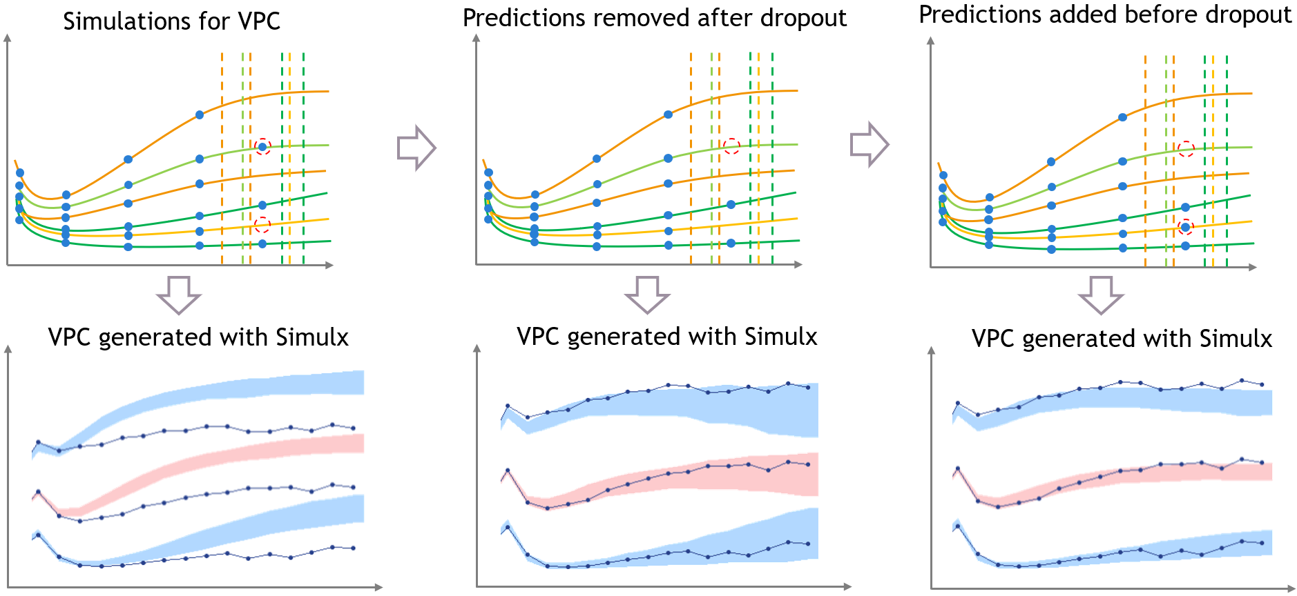
The difficulty of the approach in Step 3 is to extrapolate the design of the dataset in a way that makes sense. This can not be done in Monolix, but it has to be done in R by the user because it requires to make assumptions on the design, and it might be problematic when the design structure is complex.
For example, in the case of repeated doses, doses that are missing from the dataset because they would occur after a dropout will also have to be included in the new design. Furthermore, the user has to extrapolate the measurement times from the dataset, that are not necessarily the same for all individuals, while keeping the same measurement density for the new observations as for the rest of the observations, to avoid introducing other bias in the VPC.
Example
The example shown on this page along with the R script to correct the VPC can be downloaded here:
This example is based on simulated data from the PDTTE model developed in “Desmée, S, Mentré, F, Veyrat-Follet, C, Sébastien, B, Guedj, J (2017). Using the SAEM algorithm for mechanistic joint models characterizing the relationship between nonlinear PSA kinetics and survival in prostate cancer patients. Biometrics, 73, 1:305-312.” We assume for the sake of the example that the level of PSA is a marker of the tumour size.
6.5.2.Numerical predictive checks
Purpose
This plot displays the numerical predictive check (NPC). The NPC is a model diagnosis tool for continuous data which is closely related to the VPC procedure: the principle is similar, with a different way to visualize the resulting information. While the VPC maintains the time dimension and can be used to point out at which time points the model overpredicts or underpredicts the data, the NPC allows to compare the empirical cumulative distribution function (CDF) of the observations, computed on the original data set, with the theoretical cumulative distribution, computed from data simulated with the model of interest and the design structure of the original data set.
Note that since the NPC compares each observation with its own simulated distribution, there is no concern of data binning like for the VPC.
Examples
In the following example, the parameters of a two-compartment model with iv infusion and linear elimination are estimated on the remifentanil data set.
One can see the empirical CDF of remifentanil concentration in blue, compared to the theoretical CDF based on simulated data in black. The 90% prediction interval corresponding to the theoretical CDF is visualized as a light blue area. Discrepancies between the empirical CDF and this area are marked in red. The log-scale on the x-axis allows to focus on small observations. The plot shows that the model underpredicts small observations, and tends to overpredict some observations between 20 and 40 units.
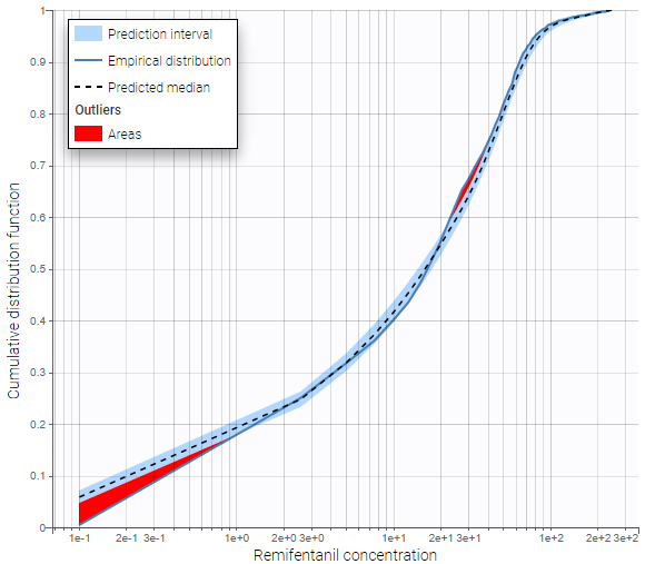
Settings
- General: Add/remove legend or grid.
- Display
- Empirical distribution: Add/remove empirical CDF.
- Predicted median: Add/remove theoretical CDF.
- Prediction interval: Add/remove the prediction interval for the theoretical CDF, and set the interpercentile level for the prediction interval (by default the level is 90) and its associated level.
- Outliers (area): Add/remove red areas indicating where the empirical CDF is outside the prediction interval.
- Calculations:
- Set the number of evaluation points in the NPC.
- Use BLQ: Choose to use BLQ data or to ignore it to compute the VPC. BLQ data can be simulated, or can be equal to the limit of quantification (LOQ). The latter case induces strong bias.
6.5.3.BLQ predictive checks
Purpose
This plot displays the proportion of censored data w.r.t. time. It is possible to choose the censoring interval. This plot is only available for projects with censored data.
Examples
The figure presents the simulated and empirical BLQ frequencies w.r.t.time (example taken from the censored1_project of the demos).
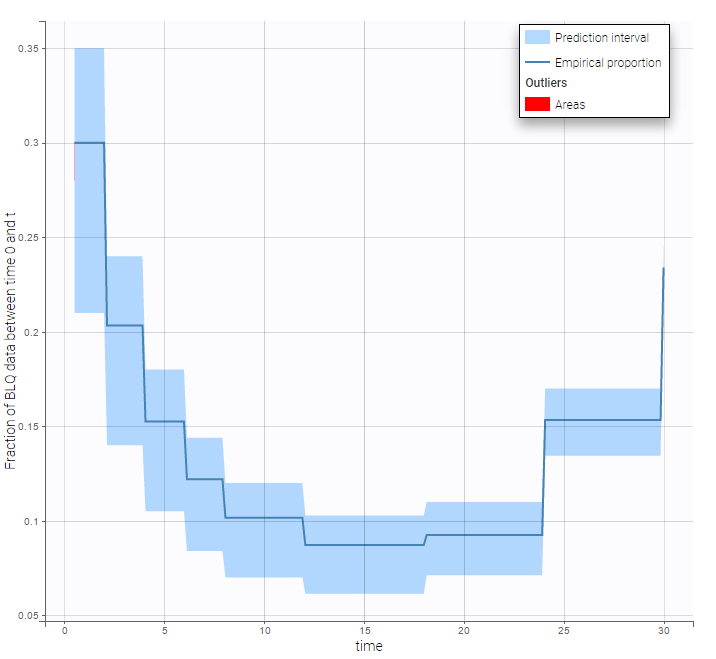
Censored interval
The censored interval can be modified in Display. By default, the limit and the censored values are used. However, one can look at a smaller censored interval for example. This is the case with the example below: on the left, the BLQ predictive check uses the default censored interval wher Min=-Infinity because there is no LIMIT column in the dataset. Since the observations are PK concentrations, Min=0 has been specified on the right, and no more outlier area is visible. This suggests that the outlier areas seen on the left are due to predicted negative values for censored observations, which means that it would be important in this case to specify a null lower limit for the censored observations by adding a column LIMIT to the dataset.
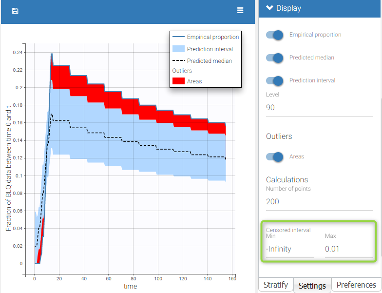 |
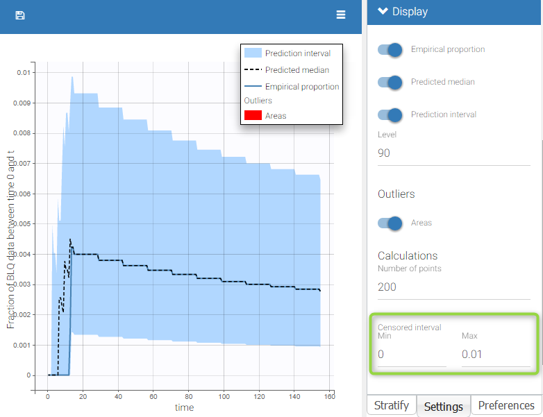 |
Settings
- General: Add/remove legend or grid
- Display
- Empirical proportion: Add/remove the blue line for empirical proportion of censored observations in cumulative observations.
- Predicted median : Add/remove the median proportion of censored observations in cumulative observations calculated by simulation.
- Prediction interval: Add/remove the prediction interval given by the model for the 90% quantile. The level (quantile) can be modified.
- Outliers (area): Add/remove red areas indicating time points for which the empirical proportion is outside the prediction interval.
- Calculations
- Number of point for the discretization
- Censored interval: min and max for censored data. By default, the limit and the censored values are used. However, one can look at a smaller censored interval for example.
By default, the censored area corresponds to the data set description and the BLQ frequency observation, the prediction interval, and the outliers are displayed.
6.5.4.Prediction distribution
Purpose
This plot displays the prediction distribution. It allows to compare the observations with the theoretical distribution of the predictions. It is based on multiple simulations of all individuals from the dataset, without the residual error. The simulations use the estimated population parameters, without considering their uncertainty.
Example
Prediction distribution plots vary slightly for different types of data. For joint models for multivariate outcomes, a separate plot is available for each type of data.
- Continuous outcomes
In the following example, the parameters of a one compartmental model with first order absorption and linear elimination are estimated on the theophylline data set. One can see the prediction distribution of the concentration overlayed with the data set.
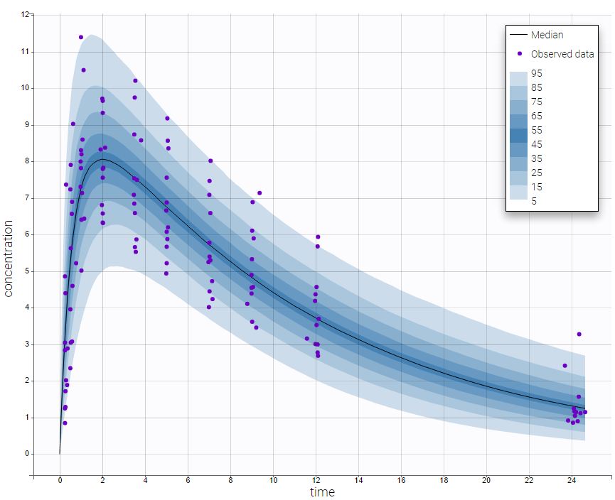
- Non-continuous outcomes: count data and categorical data
count2_project (data = ‘count2_data.txt’, model = ‘count_library/poissonTimeVarying_mlxt.txt’)
Prediction distribution plots for count data and categorical data show the predicted frequencies of the categorized data over time, computed by Monte-Carlo. In the following example, predictions come from a Poisson distribution with a time varying intensit. Note that hovering on a band reveals the corresponding modality.
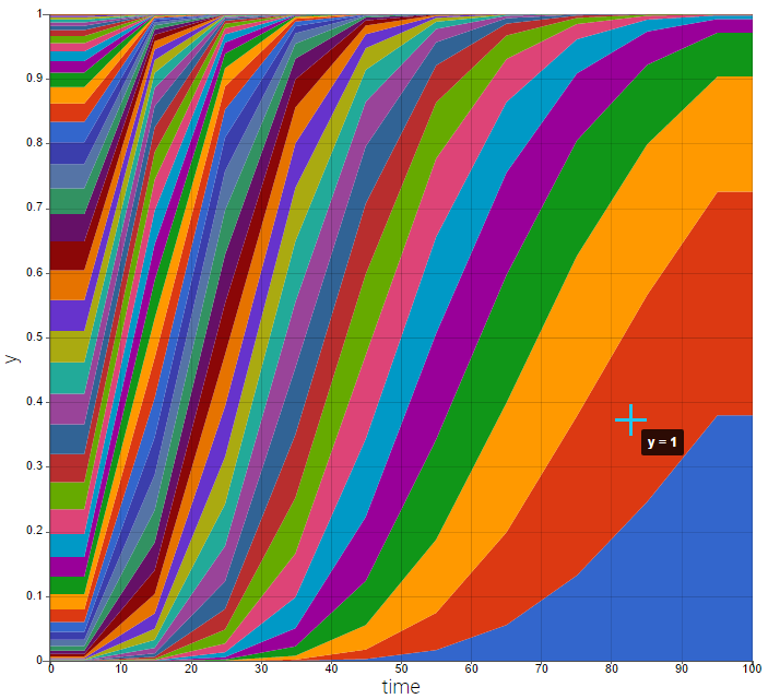
Settings
- General: Add/remove legend or grid
- Display (for continuous data)
- Observed data
- BLQ: Add/remove BLQ data if present.
- Median: Add/remove the median of predictions.
- Level: set the level (90 by default). The distribution corresponds to
.
- Number of bands: set the number of bands (9 by default) and the associated percentile in case of a discrete representation
- X Bins (for discrete data)
- Bin values: Add/remove vertical lines on the plot to indicate the bins.
- Bining criteria: Choose the bining criteria among equal width (default), equal size or least-squares
- Number of bins: Choose a fixed number of bins or a range for automatic selection, and a range for the number of data points per bin.
![[50-\frac{level}{2}, 50+\frac{level}{2}]](http://s0.wp.com/latex.php?latex=%5B50-%5Cfrac%7Blevel%7D%7B2%7D%2C+50%2B%5Cfrac%7Blevel%7D%7B2%7D%5D&bg=ffffff&fg=000&s=0 "[50-\frac{level}{2}, 50+\frac{level}{2}]") .
.By default, only the prediction distribution and the median are displayed (for continuous data).
6.6.Convergence diagnosis
6.6.1.SAEM
Purpose
This plot displays the sequence of estimates for population parameters computed after each iteration of the SAEM algorithm. The purpose is to check the convergence of the algorithm. In addition, a convergence indicator gives the estimation for -2 x log-likelihood along the iterations.
Example
In the following example, the parameters of a one-compartment model with first-order absorption and linear elimination are estimated on the theophylline data set. The vertical line indicates where the algorithm switches from the first phase to the second. Notice also that the convergence indicator is displayed. More details on the convergence indicator can be found here.
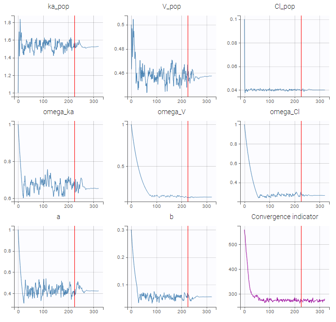
Settings
- Select plots and arrange layout. It is convenient when there are many parameters and the user wants to focus on some particular parameter convergence for example.
By default, 12 parameters are displayed.
6.6.2.MCMC
Purpose
This plot displays the sequence of estimates for the conditional means and the conditional standard deviations along the iterations of the MH algorithm during individual parameters estimation by MCMC. The purpose is to check the convergence of the algorithm. The algorithm stops when these sequences remain in an interval of a given amplitude for a certain number of iterations: this interval is visualized on the figure with horizontal lines. The plot is shown and interactively updated while the task is running, and can be found after the end of the task in the Plots frame.
Example
In the following example, the parameters of a one-compartment model with first-order absorption and linear elimination are estimated on the theophylline data set.
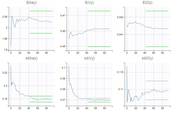
Settings
- Select plots and arrange layout. It is convenient when there are many parameters and the user wants to focus on some particular parameter convergence for example.
By default, 12 parameters are displayed.
6.6.3.Importance sampling
Purpose
This plot displays the sequence of estimates for observed log-likelihood computed by Monte Carlo approach. The purpose is to check the convergence of the algorithm.
Example
In the following example, the parameters of a three-compartments infusion model with linear elimination are estimated on the remifentanil data set. As explained on this page, the bias of the log-likelihood estimator decreases with the number of iterations, before the estimation value stabilizes. The number of points in the plot is usually smaller than the number of iterations, and depends on the total number of observations.
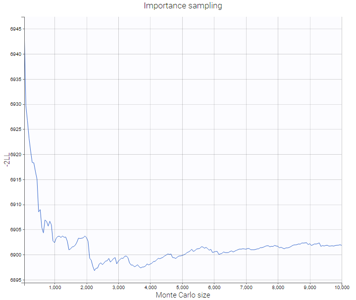
Settings
- Add/remove grid.
6.7.Tasks results
6.7.1.Likelihood contribution
Purpose
This plot displays the contribution of each individual to the log-likelihood. It is only available if the log-likelihood was previously computed. It can be sorted by index or by log-likelihood value (either via linearization of importance sampling, depending on which has been computed).
Example
In the following example, the parameters of a one-compartment model with first-order absorption, linear elimination and a delay are estimated on the warfarin data set. The figure shows the top ten contributions from individuals to the log-likelihood, computed via linearization or importance sampling methods. All the contributions appear in small size on the mini-plot on top, as well as a window indicating the selection of individuals for the main histogram.
Here we notice that the subject with id 8 has a much higher contribution to the log-likelihood than all other subjects, meaning that its reponse is less well captured by the model than others. It is worth checking this individual in the plots of individual fits, and remove it from the data set if its observations look abnormal.

Settings
- General. Add/remove the legend, grid, or a mini-plot that allows to select a range of ranks to display.
- Methods. Add/remove histograms bins for values computed by linearization or importance sampling, if they have been computed.
- Sorting. The user can choose to sort the histogram by index, or by contribution value computed with linearization or importance sampling, if they have been computed.
- Label. The user can choose to display labels on top of the bins to indicate subject indices or names (ids).
6.7.2.Standard errors of the estimates
Purpose
This plot displays a histogram with the relative standard error of each parameter estimate, computed with the Fisher Information Matrix. It is only available if the standard errors were previously computed, and it provides a graphical representation of the information already available in the column “R.S.E (%)” in the Pop.Param tab of the Results frame.
Example
In the following example, the parameters of a one-compartment model with first-order absorption, linear elimination and a delay are estimated on the warfarin data set. The figure shows the relative standard errors of all population estimates, computed via linearization and importance sampling methods, with the exact values written in front of each bin.
This figure allows here to highlight beta_Cl_tsex_F as an estimate associated with a high standard error. This suggests to check the relevance of this covariate effect, by looking at the estimate for this parameter and the result of the Wald test in the statistical tests.

Settings
- General. Add/remove the legend or grid.
- Methods. Add/remove histograms bins for values computed by linearization or stochastic approximation, if they have been computed.
7.Reporting
Starting from the 2023R1 version of the MonolixSuite, Monolix includes a feature of automated report generation. This feature is available in Monolix through Export > Generate report. After defining settings in the window that pops up and clicking on the Generate report button, a report in the form of a Microsoft Word (docx) document will be generated in the specified directory. Note that reports generated using command line and lixoftConnectors will contain tables but no plots. Reporting module is not available on CentOS 7.
Here we explain:
Report generation strategies
When selecting Export > Generate report…, there are two different strategies available for report generation:
- Using a default template file – choosing this option will generate the report containing tables of estimated population parameters (with standard errors) and log-likelihood and information criteria, as well as all plots available in the interface using their current settings. This option allow to obtain a basic report with all results in one click.
- Using a custom template file – if users choose this option, they will be required to provide a path to the template word file which contains placeholders that will be replaced by tables, plots and keywords when generating the report.
Several other options are available in the pop-up window after the Generate report option is clicked on:
- Document watermark – users can specify a custom text that will appear as a watermark in the report. Font family, font size, color, layout and transparency can be specified, if text is entered into the Text input widget.
- Generated report file – users can choose if the generated report will be saved next to the project file (in that case only the name of the generated report file needs to be given to Monolix) or in a custom directory (absolute path that includes the generated report file name needs to be given).
- Table styles (only when the custom template file option is selected) – users can choose a style for tables from the list of styles available by default in Microsoft Word. This setting can be overridden by specifying the style directly in the table placeholder. This way custom user-created or company-specific styles can be used.
Default template file
Selecting the option to use the default template file to generate a report gives users a possibility to quickly generate a document containing results of an analysis.
Such a report will consist of:
- name of the Monolix project
- data set file name,
- a date of report generation,
- a table of estimated population parameters (with standard errors, if calculation of SE was performed),
- a table of log-likelihood and information criteria (if calculation of likelihood was performed),
- all plots displayed in the GUI with settings currently defined in the interface.
By clicking on View default template, a Word document containing placeholders for all the elements that will be present in the generated report can be downloaded. This document can then be used as a basis for the creation of a custom template file.
Custom template file
The option to use the custom template file can be selected if a user has previously created a Word document (a template) that typically contains placeholders to be replaced by project-specific information, such as tables of results, plots or settings used in a project. Placeholders are strings with a specific syntax that define the settings and layout with which tables and plots will be generated during the report generation process.
For example, in the picture below, a template file on the right contains a placeholder for the observed data plot. So, after report generation, the report file on the right contains a plot for the observed data instead of this placeholder.

Using placeholders
There are three types of placeholders that can be used:
Placeholders for project settings are of format %keyword% and, during the report generation step, they will be replaced by project or global Monolix settings. For example, if a custom template file contains the placeholder %SAEM_nbBurningIterations%, this placeholder will be replaced by the number of SAEM burning iterations used by a Monolix project for which the report is being generated. The list of all project settings placeholders can be found here.
Placeholders for plots are of format <lixoftPLH>settings</lixoftPLH> and, during the report generation step, they will be replaced by plots that are available in the Monolix user interface. Placeholders for plots contain settings that describe how the generated plots should look like. All settings that are available for plots in the interface are available in reporting as well, with addition of several others that describe plot dimensions and display of captions. The list of the main plot settings placeholders can be found here.
Placeholders for tables are also of format <lixoftPLH>settings</lixoftPLH>. Placeholders for tables contain settings that describe how the generated table should look like and they allow more flexibility in the layout compared to the display of tables in the GUI. Indeed, table placeholders can contain settings that result in generated tables being different from the ones available in the Results tab of the Monolix interface, such as an option to choose which rows or columns to include in the table, or to split tables in a different direction that the one present in interface. Here is the list of all settings that can be used for table placeholders.
Placeholders do not need to be written by the users. They can be generated through the interface, using the Copy reporting placeholder (![]() ) button which can be found next to every plot and results table. Clicking on this button will display the corresponding placeholder in a pop-up window. The displayed placeholder can then be copied to a template file and will be replaced by the table or plot, exactly as they are shown in the interface, with all stratification options and display settings applied.
) button which can be found next to every plot and results table. Clicking on this button will display the corresponding placeholder in a pop-up window. The displayed placeholder can then be copied to a template file and will be replaced by the table or plot, exactly as they are shown in the interface, with all stratification options and display settings applied.
Let’s take a look at how “Copy reporting placeholder” buttons work on a specific example. If we load the demo project_censoring.pkx, go to the Observed data plot and click on the Copy reporting placeholder button above the plot, a pop-up window will appear containing the placeholder for the plot, which can then be used in a report template to generate the plot that looks exactly like the plot currently shown in the interface. As you can see on the screenshot below, the placeholder contains information about plot type, plot size, caption and axes labels.


If we now close the pop-up, enable legend and open the pop-up again, the placeholder will contain the enabled legend setting and, if we put the placeholder in a report template, the generated plot will have a legend present in its corner, as shown in the screenshot on the right.


If we would like our report to have the Observed data plot stratified by a categorical covariate, SEX, we can stratify the plot in the interface and click on the Copy reporting placeholder button again to generate a placeholder for this plot, as shown on the images below. You can notice that the generated placeholder now contains settings stratification and layout, which control stratification and plot layout.


There are several options present inside the “Placeholder for Report Template” pop-up:
- indent – determines number of spaces used for indentation of settings in the placeholder,
- flow level – determines the compactness of placeholders, i.e how often we start a new line (lower the number, more compact the placeholder will be),
- dimensions units – gives the ability to choose if width and height will be in cm or inches,
- lock aspect ratio – if on, changing width or height will change the other dimension to keep the aspect ratio present on the screen.
It is possible to edit placeholders directly inside the pop-up. Clicking on the Preview button will generate and open a Word document containing a plot or a table described with the placeholder. This option is especially useful when a user manually modifies placeholders, to check if the syntax and the behavior are correct.
Copy to clipboard button will copy the placeholder with the <lixoftPLH> tag, ready to be pasted to the custom Word template.
Using areTaskResultsAvailable
Besides placeholders, templates can include the areTaskResultsAvailable tag, which can be used to display part of the template conditionally in the report.
For example, if a template contains the text:
<? areTaskResultsAvailable(likelihood) ?>
Show this if likelihood estimation has been run
</?>
The text “Show this if likelihood estimation has been run” will be present in the generated report, only if results of the likelihood task are available, otherwise the tags and the text will not be present in the generated report. Besides text, it is possible to include placeholders inside the areTaskResultsAvailable tag. The syntax of areTaskResultsAvailable tag is areTaskResultsAvailable(task, method), with the method argument being optional. Tasks that can be used inside the parentheses are:
populationParameters,individualParameters(methods:modeandmean),correlationMatrix(methods:stochasticApproximationandlinearization),likelihood(methods:importanceSamplingandlinearization).
It is also possible to show content when task results are not available by writing !areTaskResultsAvailable.
Example use of a custom template
Download custom template for Warfarin case study
Here is an example custom template to use with the warfarin project available in demo projects (Monolix Demos > 1.1.libraries of models > warfarinPK_project.mlxtran). This dataset is also the topic of a video explaining the typical workflow in Monolix here. The custom template includes table of contents for tables and figures, which get updated when generating the report.
Renamings
A section Reporting placeholder entry renamings in Preferences can be used to change words and phrases that will appear in generated reports by default. For example, if we give alias “Thetas” to the placeholder entry “fixedeffects”, the word “fixedeffects” in the population parameter table generated by the reporting feature will be replaced by the word “Thetas”.
In addition, it is possible to rename words found in generated tables, by specifying an argument renamings inside the placeholder. This allows users to change words present in the data set as well. For example, if an imported data set contains a column “Formulation” with values T (for the test drug) and R (for the reference drug), specifying the following inside a placeholder will replace all occurrences of word “T” inside the table with “test” and “R” with “reference”:
renamings:
    T: test
    R: reference
For categorical covariates, it is possible to specify both the covariate name and the covariate modality to be replaced, in order to avoid ambiguities if, for example, category “0” appears in several covariates. In addition, quotes can be used if spaces are needed within the springs:
renamings:
    SEX#0: Male
    SEX#1: Female
    RACE#0: Caucasian
    RACE#1: "African american"
    RACE#2: Hispanic
Respecting the indentation before the modalities to replace and the space after the “:” is crucial to have the placeholder properly recognized.
Generating reports from the command line
It is possible to generate a report directly from R with the connector generateReport() or through the command line, without using the Monolix interface. This can be useful when running Monolix on a server.
To generate a report via command line, the executable reportGenerator can be called from the lib folder (typically $HOME/Lixoft/MonolixSuite2023R1/lib/):
reportGenerator -p monolix_project_path
Multiple options can be provided to reportGenerator:
| -?, -h, –help | Displays the help. |
| -p, –project <path> | Project file to load |
| –tpl, –template <path> | Template .docx file used as reporting base (if not provided a default report file is generated) |
| –onxt, –output-next-project <[true], false> | Generate report next to project |
| –op, –output-path <path> | Generated report file name (if output-next-project is true) or complete path (if output-next-project is false) |
| –tab, –tables-style <style> | Table style sheet applied on generated tables |
| –wt, –watermark-text <text> | Watermark text |
| –wff, –watermark-font-family <[Arial], …> | Watermark font family |
| –wfs, –watermark-font-size <integer> | Watermark font size |
| –wc, –watermark-color <[255:0:0]> | Watermark color (RGB) |
| –wl, –watermark-layout <[horizontal], diagonal> | Watermark layout |
| –wst, –watermark-semi-transparent <[true], false> | Watermark semi-transparent |
7.1.Reporting examples
NCA summary table split by a covariate
- example: demo project_Theo_extravasc_SS.pkx
<lixoftPLH>
data:
    task: nca
    metrics: [Nobs, mean, CV, min, median, max]
    parameters: [Cmax, AUClast, CLss_F, Vz_F, HL_Lambda_z]
display:
    units: true
    inlineUnits: true
    metricsDirection: horizontal
    significantDigits: 4
    fitToContent: true
stratification:
    state: {split: [FORM]}
    splitDirection: [h]
</lixoftPLH>
BE table for absolute bioavailability
- example: demo project_parallel_absBioavailability.pkx
<lixoftPLH>
data:
    task: be
    table: confidenceIntervals
    metrics: [Ratio, CILower, CIUpper]
    parameters: [AUCINF_obs, AUClast]
display:
    units: true
    inlineUnits: true
    significantDigits: 4
    fitToContent: true
renamings:
    bioequivalence: "Relative bioavailability (%) based on:"
    CILower: "Lower 90% CI"
    CIUpper: "Upper 90% CI"
</lixoftPLH>
Table of NCA settings
- example: demo project_censoring.pkx
| Data type | %data_type% |
| Dose type | %NCA_administrationType% |
| Weighting for λz slope calculation | %NCA_lambdaWeighting% |
| Point selection method for λz slope calculation | %NCA_lambdaRule% |
| AUC calculation method | %NCA_integralMethod% |
| BLQ before Tmax treated as | %NCA_blqMethodBeforeTmax% |
| BLQ after Tmax treated as | %NCA_blqMethodAfterTmax% |
Individual NCA parameters for a group
- example: demo DoseAndLOQ_byCategory.pkx
<lixoftPLH>
data:
    task: nca
    metrics: [ID]
    parameters: [AUCINF_D_obs, AUCINF_obs, AUClast, AUClast_D, Cmax, Cmax_D, Tmax]
display:
    units: true
    inlineUnits: true
    metricsDirection: vertical
    significantDigits: 2
    fitToContent: true
stratification:
    state: {split: [STUDY], filter: [[STUDY, [1]]]}
    splitDirection: [v]
</lixoftPLH>
NCA summary table with summary metrics filtered by group
- example: demo DoseAndLOQ_byCategory.pkx
<lixoftPLH>
data:
    task: nca
    metrics: [Nobs, mean, SE, CV, min, median, max, geoMean, harmMean]
    parameters: [AUCINF_D_obs, AUCINF_obs, AUClast, AUClast_D, Cmax, Cmax_D, Tmax]
display:
    units: true
    inlineUnits: true
    metricsDirection: vertical
    significantDigits: 2
    fitToContent: true
stratification:
    state: {split: [STUDY], filter: [[STUDY, [1]]]}
    splitDirection: [v]
</lixoftPLH>
Individual covariate table
- example: demo project_M2000_bolus_SD.pkx
<lixoftPLH>
data:
    task: nca
    metrics: [ID]
    excludedParameters: all
    covariates: all
    covariatesAfterParameters: true
display:
    units: true
    inlineUnits: true
    metricsDirection: vertical
    significantDigits: 4
    fitToContent: true
</lixoftPLH>
Included in LambdaZ table
- example: demo project_censoring.pkx
<lixoftPLH>
data:
    task: nca
    metrics: [ID]
    excludedParameters: all
    covariates: all
    covariatesAfterParameters: true
display:
    units: true
    inlineUnits: true
    metricsDirection: vertical
    significantDigits: 4
    fitToContent: true
</lixoftPLH>
7.2.List of reporting keywords
This page provides a list of placeholders for project settings that can be used in report templates for Monolix projects.
| Keyword | Description | Possible values |
| %SAEM_nbBurningIterations% | Number of iterations in the burn-in phase. | a number |
| %SAEM_nbExploratoryIterations% | If “exploratoryAutoStop” is set to FALSE, it is the number of iterations in the exploratory phase. Else, if “exploratoryAutoStop” is set to TRUE, it is the maximum of iterations in the exploratory phase. | a number |
| %SAEM_exploratoryAutoStop% | Whether exploratory autostop was used. | used / not used |
| %SAEM_exploratoryInterval% | Minimum number of interation in the exploratory phase. | a number |
| %SAEM_nbSmoothingIterations% | If “smoothingAutoStop” is set to FALSE, it is the number of iterations in the smoothing phase. Else, if “smoothingAutoStop” is set to TRUE, it is the maximum of iterations in the smoothing phase. | a number |
| %SAEM_smoothingAutoStop% | Whether smoothing autostop was used. | used / not used |
| %SAEM_smoothingInterval% | Minimum number of interation in the smoothing phase. Used only if “smoothingAutoStop” is TRUE. | a number |
| %SAEM_simulatedAnnealing% | Whether simulated annealing was used. | used / not used |
| %SAEM_decreasingRateResError% | Simulated annealing decreasing rate for the variance of the residual errors. | a number |
| %SAEM_decreasingRateIndivParam% | Simulated annealing decreasing rate for the variance of the individual parameters. | a number |
| %SAEM_withoutVariabilityMethod% | Method for parameters without variability. | variability at first stage / decreasing variability / no variability |
| %CondDist_nbMaxIterations% | Maximum number of iterations for conditional distribution sampling. | a number |
| %CondDist_nbSimulatedParameters% | Number of samples from the conditional distribution per individual. | a number |
| %CondDist_intervalLength% | Interval length for MCMC convergence assessment. | a number |
| %CondDist_relIntervalWidth% | Relative interval width for MCMC convergence assessment. | a number |
| %EBEs_nbMaxIterations% | Maximum number of optimization iterations for EBEs task. | a number |
| %EBEs_optimizationTolerance% | Optimization tolerance for EBEs task. | a number |
| %SE_nbMaxIterations% | Maximum number of optimization iterations for Standard Errors task. | a number |
| %SE_nbMinIterations% | Minimum number of optimization iterations for Standard Errors task. | a number |
| %LL_nbFixedIterations% | Monte Carlo size for the LL task. | a number |
| %LL_degreesFreedom% | Degrees of freedom of the t-distribution. | 5 (fixed) or 1, 2, 5, 10 (optimized) |
| %Global_seed% | Seed used in the project. | a number |
| %MCMC_transitionKernels% | Number of calls for each one of the three MCMC kernels. | number-number-number (e.g., 2-2-2) |
| %MCMC_acceptanceRatio% | Target acceptance ratio for MCMC. | a number |
| %MCMC_nbChains% | Computed number of chains if not automatically set. | a number |
| %MCMC_minIndivForChains% | Minimum number of individuals for chains if automatically set. | a number |
| %TotalNbSubjects% | Total number of subjects in the data set (all observation ids together). | a number |
| %TotalNbSubjectsOcc% | Total number of subjects-occasions in the dataset (all observation ids together). | a number |
| %AvgNbDosesPerSubject% | Average number of doses per subject (any administration id, any occasion, all observation ids). | a number |
| %TotalNbObservations% | Total number of observations in the data set. | if one obs id, number, if several obs id, PK: xx, PD: xx |
| %AvgNbObservationsPerID% | Average number of observations per id (all occasions together). | if one obs id, number, if several obs id, PK: xx, PD: xx |
| %MinNbObservationsPerID% | Minimum number of observations per id (all occasions together). | if one obs id, number, if several obs id, PK: xx, PD: xx |
| %MaxNbObservationsPerID% | Maximum number of observations per id (all occasions together). | if one obs id, number, if several obs id, PK: xx, PD: xx |
| %PercentCensoredObservations% | Percentage of censored observations. | if one obs id, number, if several obs id, PK: xx, PD: xx |
| %StructModelCode% | Mlxtran code for the structural model. | whole structural model file content, as shown in the Structural model tab |
| %reportGenerationDateTime(yyyy-MM-dd HH:mm:ss)% | Report generation date and time. Part of yyyy-MM-dd HH:mm:ss can be removed or reordered. | yyyy-MM-dd HH:mm:ss |
| %system% | Operating system on which report was generated. | Linux, macOS, Windows |
| %version% | Version of Monolix with which report was generated. | 2023R1 |
| %project_fileName% | File name of the project (without path). | Example: NCA_run.pkx |
| %project_filePath% | File path of the project. | Example: C:/Users/user/lixoft/monolix/monolix2024R1/demos/1.creating_and_using_models/1.1.libraries_of_models/theophylline_project.mlxtran |
| %data_fileName% | File name of the data set (without path). | Example: data.csv |
7.3.List of plot settings
This page describes all the settings that can be used in plot placeholders and are not editable by changing settings in the interface. All of them are optional (default values are described in the Default column).
| Setting | Group | Default | Possible values | Description | Example |
| widthCm | – | 16 | positive numbers | Width of the plot in the report document in centimetres. | widthCm: 16 |
| widthInches | – | 6.3 | positive numbers | Width of the plot in the report document in inches. | widthInches: 6.3 |
| heightCm | – | 11.1 | positive numbers | Height of the plot in the report document in centimetres. | heightCm: 11.09 |
| heightInches | – | 4.37 | positive numbers | Height of the plot in the report document in inches. | heightInches: 4.37 |
| zoom | – | 100 | positive numbers | Larger values will increase the label font sizes and margins. | zoom: 80 |
| caption | – | no caption | a phrase | Caption that will appear next to the plot. | caption: Individual fits |
| captionAbove | – | false | true, false | If true, caption will be positioned above the plot. If false, caption will be positioned below the plot. | captionAbove: true |
| legendPosition | settings | ne | n, ne, e, se, s, sw, w, nw | Position of the legend, based on abbreviations of compass points. | legendPosition: sw |
For all other settings, select the settings of your plot in the GUI and then click the “copy placeholder” button to see the corresponding placeholder.
7.4.List of table placeholder settings
The following page describes all the settings that can be used in table placeholders in reporting templates. Placeholders for tables can include four different groups of settings. These are:
- “data” (required) – containing settings about table content, such as type of the table, and rows and columns that the table will contain,
- “display” (optional) – containing information about table display (e.g., number of significant digits to which the values in the table should be rounded, table direction, style, …),
- “renamings” (optional) – containing various words present in the data set or Monolix that should be reworded in the table.
Settings inside these groups of settings need to be indented or put inside curly brackets. It is crucial to respect the indentation rules and the space after the “:” for the placeholder to be properly interpreted.
Data
Data settings define the type of the table that will be generated, as well as rows and columns that the table will contain. Here is the list of all settings of the data group of settings, along with their descriptions:
| Setting | Table | Required |
Possible values | Description |
| task | All | yes | populationParameters, individualParameters, correlationMatrix, likelihood | Task of which the table represents the results. |
| table | Likelihood and SE tables | no | Likelihood: criteria/samplingInformation SE: matrix/eigenvalues |
Table type. If empty, criteria or matrix table will be generated, depending on the task. |
| methods | Population parameters and likelihood | no (default: all) | Population parameters: linearization, stochasticApproximation, all Likelihood: linearization, importanceSampling, all |
Value for population parameters is used for the SE part of the table. |
| method | Individual parameters and SE | yes | Individual parameters: mode, mean SE: linearization, stochasticApproximation |
Method for reported values. |
| metrics | Population parameters table | no | SE, RSE, CV, SHRINKAGE, all | If equal to “all”, all available rows or columns will be present in the table. If specific metrics are given, only those rows/columns will be available in the table. |
| metrics | Individual parameters table | no | ID, MIN, Q1, MEDIAN, Q3, MAX, SHRINKAGE, all | If equal to “all”, all available rows or columns will be present in the table. If specific metrics are given, only those rows/columns will be available in the table. |
| metrics | SE tables | no | Matrix table: RSE Eigenvalues table: MIN, MAX, Ratio, all |
If equal to “all”, all available rows or columns will be present in the table. If specific metrics are given, only those rows/columns will be available in the table. |
| metrics | Likelihood tables | no | Criteria table: OFV, AIC, BIC, BICc, all | If equal to “all”, all available rows or columns will be present in the table. If specific metrics are given, only those rows/columns will be available in the table. |
| excludedMetrics | All | no (default: none) | Same arguments as for metrics (except “all”). | Metrics that will be excluded from the table. Handy when a user wants to specify metrics: “all” and exclude a few with excludedMetrics. |
| parameters | All except SE tables | no (default: all) | Model parameter names, or all. | Parameters that will be included in the table. |
| excludedParameters | All except SE tables | no (default: none) | Model parameter names, or all. | Parameters that will be excluded from the table. |
| ids | Individual parameters | no (default: all) | One or several of IDs present in the dataset, or “all”. | IDs of subjects whose parameters should be shown in the table. The summary statistics will be calculated on all individuals, not just ones shown in the table. If not present, default is “all”. |
| excludedIds | Individual parameters | no (default: none) | Same arguments as for ids, excluding “all”. | IDs of subjects whose parameters should be excluded from the table. The summary statistics will be calculated on all individuals, not just ones shown in the table. |
| nbOccDisplayed | Individual parameters | no (default: -1 meaning all) | -1 or an integer | -1 means all occasion levels are diplayed. 0 mean none of the occasion levels are diplayed. 1 means only the first occasion level is displayed, etc. |
| covariates | Individual parameters | no (default: all) | One or more of covariates present in the data set, or “all”. | Which covariates to include in the table. |
| covariatesAfterParameters | Individual parameters | no (default: true) | true, false | If covariates should be shown after parameters in the table. |
| types | Population parameters table | no (default: all) | One or more of: fixedEffects, stDev, correlations, error, all | Which types of parameters should be included in the table (fixed effects, standard deviations of random effects, correlations, error model parameters). |
Display
Display group of settings defines how the information in the tables will be displayed. Here is the list of all settings for the display group of settings:
| Setting | Table | Required | Possible values | Description | Example(s) |
| style | All | no (default: selected in Generate report pop-up) | Name of table styles present in the template document. | Microsoft Word document template style to apply to the table. This setting overrides the setting in the Generate report pop-up. | style: “Medium Grid 1 – Accent 1” |
| metricsDirection | All | no (default: vertical) | vertical, horizontal | Direction of metrics. | metricsDirection: horizontal |
| significantDigits | All | no (default: taken from Preferences) | positive integers | Number of significant digits values in the table will be rounded to. | signifcantDigits: 3 |
| trailingZeros | All | no (default: taken from Preferences) | true, false | If trailing zeros should be shown in the tables. | trailingZeros: true |
| fitToContent | All | no (default: true) | true, false | If true, width of the table will be equal to the width of content, otherwise width of the table will be equal to the width of the page. | fitToContent: false |
| caption | All | no (default: no caption) | a phrase inside quotation marks | Caption that will appear next to the table. | caption: “EBEs” |
| captionAbove | All | no (default: false) | true, false | If true, caption will be positioned above the table. If false, caption will be positioned below the table. | captionAbove: true |
| fontSize | All | no (default: 12) | a number | Font size of the table content (will not be applied to the caption). | fontSize: 10 |
| colored | SE matrix table | no (default: true) | true, false | If values should be color-coded. | colored: false |
Renamings
Renamings setting can be provided to the placeholder to replace certain words or expressions that will appear in the table with a user-defined word or expression. We will explain the usage of renamings setting on a concrete example.
Let’s take a look at the demo project iov1_project.mlxtran. Let’s say we want to put a table of EBEs in the report, with renaming of the occasion column header.
A generated placeholder for the EBEs table, with its default settings, is shown below, including the table it generates.
<lixoftPLH>
data:
    task: individualParameters
    method: mode
    metrics: [ID]
    parameters: all
    covariates: all
    covariatesAfterParameters: true
display:
    significantDigits: 4
    fitToContent: true
    metricsDirection: vertical
</lixoftPLH>
| ID | OCC | ka | V | Cl | SEX | TREAT |
| 1 | 1 | 1.6102 | 0.443 | 0.03353 | M | A |
| 1 | 2 | 1.6102 | 0.3498 | 0.03353 | M | B |
| 2 | 1 | 1.4346 | 0.4941 | 0.02389 | M | A |
| 2 | 2 | 1.4346 | 0.4018 | 0.02389 | M | B |
| 3 | 1 | 1.8029 | 0.5139 | 0.03806 | M | A |
| 3 | 2 | 1.8029 | 0.4048 | 0.03806 | M | B |
| 4 | 1 | 0.9828 | 0.4857 | 0.03621 | M | A |
| 4 | 2 | 0.9828 | 0.3875 | 0.03621 | M | B |
| 5 | 1 | 1.8905 | 0.5514 | 0.03684 | M | A |
| 5 | 2 | 1.8905 | 0.4388 | 0.03684 | M | B |
| 6 | 1 | 1.3289 | 0.4653 | 0.03175 | M | A |
| 6 | 2 | 1.3289 | 0.3623 | 0.03175 | M | B |
| 7 | 1 | 1.9682 | 0.3904 | 0.04016 | M | B |
| 7 | 2 | 1.9682 | 0.509 | 0.04016 | M | A |
Let’s say we would like to hide some of the columns (SEX) and rename some of the expressions in the table. For example, it would be convenient to rename “OCC” to “Period”. We can then modify the placeholder to look like the one on the left and it will generate the table on the right.
<lixoftPLH>
data:
    task: individualParameters
    method: mode
    metrics: [ID]
    parameters: all
    excludedCovariates: SEX
    covariatesAfterParameters: true
display:
    significantDigits: 4
    fitToContent: true
    metricsDirection: vertical
renamings:
    OCC: "Period"
</lixoftPLH>
| ID | Period | ka | V | Cl | TREAT |
| 1 | 1 | 1.6102 | 0.443 | 0.03353 | A |
| 1 | 2 | 1.6102 | 0.3498 | 0.03353 | B |
| 2 | 1 | 1.4346 | 0.4941 | 0.02389 | A |
| 2 | 2 | 1.4346 | 0.4018 | 0.02389 | B |
| 3 | 1 | 1.8029 | 0.5139 | 0.03806 | A |
| 3 | 2 | 1.8029 | 0.4048 | 0.03806 | B |
| 4 | 1 | 0.9828 | 0.4857 | 0.03621 | A |
| 4 | 2 | 0.9828 | 0.3875 | 0.03621 | B |
| 5 | 1 | 1.8905 | 0.5514 | 0.03684 | A |
| 5 | 2 | 1.8905 | 0.4388 | 0.03684 | B |
| 6 | 1 | 1.3289 | 0.4653 | 0.03175 | A |
| 6 | 2 | 1.3289 | 0.3623 | 0.03175 | B |
| 7 | 1 | 1.9682 | 0.3904 | 0.04016 | B |
| 7 | 2 | 1.9682 | 0.509 | 0.04016 | A |
8.Export a Monolix project to PKanalix and Simulx
Export a Monolix project to PKanalix, Simulx and Sycomore
MonolixSuite applications are interconnected and projects can be exported/imported between different applications. This interconnection is guaranteed by using the same model syntax (mlxtran language) and the same dataset format. You can export a Monolix project to PKanalix or Simulx in one click directly from the interface.
To export a project click EXPORT PROJECT TO in the top menu “Export”:
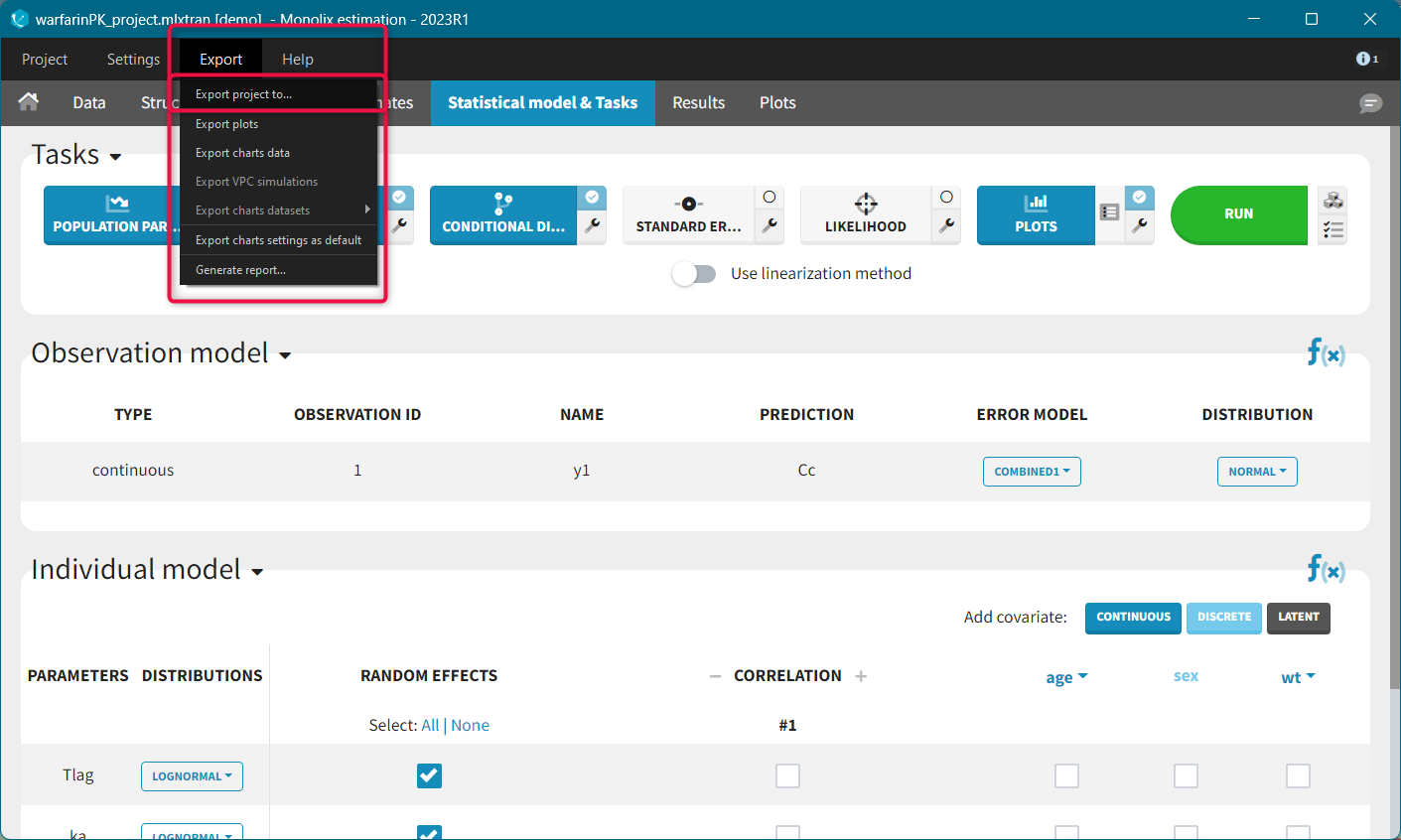
The export pop-up window will appear where you can choose:
- to which application you want to export your current project: PKanalix, Simulx or Sycomore (starting from the 2024 version)
- which dataset you want to use in the export (PKanalix and Simulx only): original dataset, vpc dataset (if VPC plot has been generated), individual fits dataset (if individual fits plot has been generated)
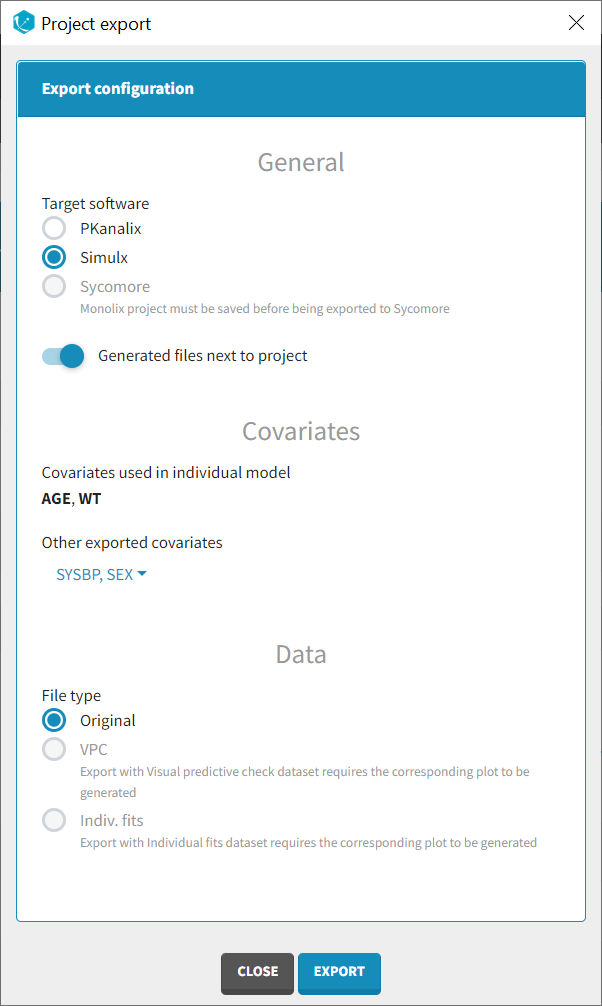
By default, Monolix will copy all files, e.g. dataset and model, next to the new PKanalix/Simulx project. To keep current location of these files, switch the toggle “Generated files next to project” off.
It is now feasible to export additional covariates to Simulx that were not initially included in the individual model (starting from version 2024R1). In the export configurations window a dedicated “Covariates” section appears. This section lists the covariates that are already incorporated in the model, and underneath, additional covariates can be selected from an available drop-down menu titeld “Other exported covariates”.
To export a Monolix project click the “EXPORT” button at the bottom. PKanalix/Simulx/Sycomore will open automatically with a predefined project called “untitled”. You can save this project, edit and run. For more information about exported elements, see:
- Import from Monolix to Simulx documentation page
- Import from Monolix to PKanalix documentation page
When exporting to Sycomore, a new Sycomore project will be created that contains only the current Monolix project. To add additional Monolix projects to the Sycomore project, the following instructions can be followed.
Share a Monolix project
The 2024 version of MonolixSuite introduces a highly convenient method for sharing projects. Simply click on “Share Project” in the export menu, and a zip folder is generated containing all the required files to re-open the project (dataset, model if not from library, mlxtran file, result folder). By default, the suggested location for the zipped shared project matches that of the original, but this can be easily modified to any other location on the computer.
The functionality of this feature remains consistent across all software within the MonolixSuite.
9.R functions to run Monolix
On the use of the R-functions
We now propose to use Monolix via R-functions. The package lixoftConnectors provides access to the project exactly in the same way as you would do with the interface. All the installation guidelines and initialization procedure can be found here. All the functions of lixoftConnectors are described below. To go beyond what the interface allows, the RsSimulx package provides additional functions for automatic PK model building, bootstrap simulation and likelihood profiling, among others.
- Installation guidelines and initialization procedure
- Examples using R functions
- Load and run a project
- Convergence assessment
- Profile likelihood
- Bayesian individual dynamic predictions
- Covariate search
- Generate plots in R
- Handling of warning/error/info messages
- List of the R functions
- Description of the functions concerning the algorithm settings
- Description of the functions concerning the bootstrap
- Description of the functions concerning the convergence assessment
- Description of the functions concerning the covariate model
- Description of the functions concerning the dataset
- Description of the functions concerning the individual model
- Description of the functions concerning the initial values and estimation method
- Description of the functions concerning the initialization and path to demo projects
- Description of the functions concerning the model building tasks
- Description of the functions concerning the observation model
- Description of the functions concerning the plots
- Description of the functions concerning the project management
- Description of the functions concerning the project settings and preferences
- Description of the functions concerning the reporting
- Description of the functions concerning the results
- Description of the functions concerning the scenario
List of the R functions
Description of the functions concerning the algorithm settings
- getConditionalDistributionSamplingSettings: Get the conditional distribution sampling settings for the current project.
- getConditionalModeEstimationSettings: Get the conditional mode (EBEs) estimation settings for the current project.
- getGeneralSettings: Get a summary of the settings related to chains for Monolix algorithms for the current project.
- getLogLikelihoodEstimationSettings: Get the log-likelihood estimation settings of the current project.
- getMCMCSettings: Get the MCMC algorithm settings of the current project.
- getPopulationParameterEstimationSettings: Get the population parameter estimation settings for the current project.
- getStandardErrorEstimationSettings: Get the standard error estimation settings for the current project.
- setConditionalDistributionSamplingSettings: Set the value of one or more of the conditional distribution sampling settings for the current project.
- setConditionalModeEstimationSettings: Set the value of one or more of the conditional mode (EBEs) estimation settings for the current project.
- setGeneralSettings: Set the value of one or more of the settings related to chains for Monolix algorithms for the current project.
- setLogLikelihoodEstimationSettings: Set the value of the log-likelihood estimation settings for the current project.
- setMCMCSettings: Set the value of one or more of the MCMC algorithm settings related to transition kernels of the current project.
- setPopulationParameterEstimationSettings: Set the value of one or more of the population parameter estimation settings for the current project.
- setStandardErrorEstimationSettings: Set the value of one or more of the standard error estimation settings for the current project.
Description of the functions concerning the bootstrap
- getBootstrapResults: Get the results of boostrap.
- getBootstrapSettings: Get the settings that will be used during the run of bootstrap.
- runBootstrap: Run boostrap.
Description of the functions concerning the convergence assessment
- getAssessmentResults: Get the results of the convergence assessment.
- getAssessmentSettings: Get the current settings for running the convergence assessment.
- runAssessment: Run assessment.
Description of the functions concerning the covariate model
- addCategoricalTransformedCovariate: Create a new categorical covariate by transforming an existing one.
- addContinuousTransformedCovariate: Create a new continuous covariate by transforming an existing one.
- addMixture: Add a new latent covariate to the current model giving its name and its modality number (how many subpopulations).
- removeCovariate: Remove any of the transformed covariates (discrete and continuous) and/or latent covariates.
Description of the functions concerning the dataset
- addAdditionalCovariate: Create an additional covariate for stratification purpose.
- applyFilter: Apply a filter on the current data.
- createFilter: Create a new filtered data set by applying a filter on an existing one and/or complementing it.
- deleteAdditionalCovariate: Delete a created additinal covariate.
- deleteFilter: Delete a data set.
- editFilter: Edit the definition of an existing filtered data set.
- formatData: Adapt and export a data file as a MonolixSuite formatted data set.
- getAvailableData: Get information about the data sets and filters defined in the project.
- getCovariateInformation: Get the name, the type and the values of the covariates present in the project.
- getFormatting: Get data formatting settings from a loaded project.
- getObservationInformation: Get the name, the type and the values of the observations present in the project.
- getTreatmentsInformation: Get information about doses present in the loaded dataset.
- removeFilter: Remove the last filter applied on the current data set.
- renameAdditionalCovariate: Rename an existing additional covariate.
- renameFilter: Rename an existing filtered data set.
- selectData: Select the new current data set within the previously defined ones (original and filters).
Description of the functions concerning the individual model
- getIndividualParameterModel: Get a summary of the individual parameter model.
- getVariabilityLevels: Get a summary of the variability levels (inter-individual and/or intra-individual variability, i.
- setCorrelationBlocks: Define the correlation block structure associated to some of the variability levels of the current project.
- setCovariateModel: Set which are the covariates influencing individual parameters present in the project.
- setIndividualLogitLimits: Set the minimum and the maximum values for an individual parameter.
- setIndividualParameterDistribution: Set the distribution of the estimated parameters.
- setIndividualParameterModel: Update the individual parameter model.
- setIndividualParameterVariability: Add or remove inter-individual and/or intra-individual variability (i.
Description of the functions concerning the initial values and estimation method
- getFixedEffectsByAutoInit: Compute initial values for fixed-effect population parameters.
- getPopulationParameterInformation: Get population parameters information.
- setInitialEstimatesToLastEstimates: Set the initial value of all the population parameters in the current project to the ones previously estimated.
- setPopulationParameterInformation: Set population parameters initialization and estimation method.
Description of the functions concerning the initialization and path to demo projects
- initializeLixoftConnectors: Initialize lixoftConnectors API for a given software.
- getDemoPath: Get the path to the demo projects.
Description of the functions concerning the model building tasks
- getModelBuildingResults: Get the results of automatic covariate model building or automatic statistical model building.
- getModelBuildingSettings: Get the current settings for running model building.
- runModelBuilding: Run model building for automatic covariate model building or automatic statistical model building.
Description of the functions concerning the observation model
- getContinuousObservationModel: Get a summary of the information concerning the continuous observation statistical model(s) in the project.
- setAutocorrelation: Add or remove auto-correlation from the error model used on some of the observation models.
- setErrorModel: Set the error model type to be used for the observation model(s).
- setObservationDistribution: Set observation model distribution.
- setObservationLimits: Set observation model distribution limits for logitNormal observations.
Description of the functions concerning the plots
- plotBivariateDataViewer: Plot the bivariate viewer.
- plotCovariates: Plot the covariates.
- plotObservedData: Plot the observed data.
- plotImportanceSampling: Plot iterations of the likelihood estimation by importance sampling.
- plotMCMC: Plot iterations and convergence for the conditional distribution task.
- plotSaem: Plot iterations and convergence for the SAEM algorithm (population parameters estimation).
- plotParametersDistribution: Plot the distribution of the individual parameters.
- plotParametersVsCovariates: Plot individual parameters vs covariates.
- plotRandomEffectsCorrelation: Plot correlations between random effects.
- plotStandardizedRandomEffectsDistribution: Plot the distribution of the standardized random effects.
- plotIndividualFits: Plot the individual fits.
- plotObservationsVsPredictions: Plot the observation vs the predictions.
- plotResidualsDistribution: Plot the distribution of the residuals.
- plotResidualsScatterPlot: Plot the scatter plots of the residuals.
- plotBlqPredictiveCheck: Plot the BLQ predictive checks.
- plotNpc: Plot the numerical predictive checks.
- plotPredictionDistribution: Plot the prediction distribution.
- plotVpc: Plot the visual predictive checks.
- getPlotPreferences: Define the preferences to customize plots.
- resetPlotPreferences: Reset plot preferences to go back to default preferences.
- setPlotPreferences: Set preferences to customize plots.
Description of the functions concerning the project management
- exportProject: Export the current project to another application of the MonolixSuite, and load the exported project.
- getData: Get a description of the data used in the current project.
- getInterpretedData: Get data after interpretation done by the software, as it is displayed in the Data tab in the interface.
- getLibraryModelContent: Get the content of a library model.
- getLibraryModelName: Get the name of a library model given a list of library filters.
- getMapping: Get mapping between data and model.
- getStructuralModel: Get the model file for the structural model used in the current project.
- importProject: Import a Monolix or a PKanalix project into the currently running application initialized in the connectors.
- isProjectLoaded: Get a logical saying if a project is currently loaded.
- loadProject: Load a project in the currently running application initialized in the connectors.
- newProject: Create a new project.
- saveProject: Save the current project as a file that can be reloaded in the connectors or in the GUI.
- setData: Set project data giving a data file and specifying headers and observations types.
- setMapping: Set mapping between data and model.
- setStructuralModel: Set the structural model.
- shareProject: Create a zip archive file from current project and its results.
Description of the functions concerning the project settings and preferences
- getConsoleMode: Get console mode, ie volume of output after running estimation tasks.
- getPreferences: Get a summary of the project preferences.
- getProjectSettings: Get a summary of the project settings.
- setConsoleMode: Set console mode, ie volume of output after running estimation tasks.
- setPreferences: Set the value of one or several of the project preferences.
- setProjectSettings: Set the value of one or several of the settings of the project.
Description of the functions concerning the reporting
- generateReport: Generate a project report with default options or from a custom Word template.
Description of the functions concerning the results
- exportChartDataSet: Export the data of a chart into Lixoft suite compatible data set format.
- getCorrelationOfEstimates: Get the inverse of the last estimated Fisher matrix computed either by all the Fisher methods used during the last scenario run or by the specific one passed in argument.
- getEstimatedConfidenceIntervals: Get the confidence interval of population parameters computed either by all the Fisher methods used during the last scenario run or by the specific one passed in argument.
- getEstimatedIndividualParameters: Get the last estimated values for each subject of the individual parameters present within the current project.
- getEstimatedLogLikelihood: Get the values computed by using a log-likelihood algorithm during the last scenario run, with or without a method-based filter.
- getEstimatedPopulationParameters: Get the last estimated value of some of the population parameters present within the current project (fixed effects + individual variances + correlations + latent probabilities + error model parameters).
- getEstimatedRandomEffects: Get the random effects for each subject of the individual parameters present within the current project.
- getEstimatedStandardErrors: Get the last estimated standard errors of population parameters computed either by all the Fisher methods used during the last scenario run or by the specific one passed in argument.
- getEtaShrinkage: Get the shrinkage values for each individual parameter.
- getLaunchedTasks: Get a list of the tasks which have available results.
- getSAEMiterations: Retrieve the successive values of some of the population parameters present within the current project (fixed effects + individual variances + correlations + latent probabilities + error model parameters) during the previous run of the SAEM algorithm.
- getSimulatedIndividualParameters: Get the simulated values for each replicate of each subject of some of the individual parameters present within the current project.
- getSimulatedRandomEffects: Get the simulated values for each replicate of each subject of some of the individual random effects present within the current project.
- getTests: Get the results of performed statistical tests.
Description of the functions concerning the scenario
- computeChartsData: Compute (if needed) and export the charts data of a given plot or, if not specified, all the available project plots.
- getLastRunStatus: Return an execution report about the last run with a summary of the error which could have occurred.
- getScenario: Get the list of tasks that will be run at the next call to
runScenario. - runScenario: Run the scenario that has been set with
setScenario. - setScenario: Clear the current scenario and build a new one from a given list of tasks.
- runConditionalDistributionSampling: Estimate the conditional distribution which can be sampled from (i.
- runConditionalModeEstimation: Estimate the individual parameters using the conditional mode estimation algorithm (EBEs).
- runLogLikelihoodEstimation: Run the log-likelihood estimation algorithm.
- runPopulationParameterEstimation: Estimate the population parameters with the SAEM algorithm.
- runStandardErrorEstimation: Estimate the Fisher Information Matrix (FIM) and the standard errors of the population parameters.
[Monolix] Get conditional distribution sampling settings
Description
Get the conditional distribution sampling settings for the current project.
Associated settings are:
ratio |
(0 < double < 1) | Width of the relative interval for stopping criteria (i.e. 0.05 for 5%). |
enableMaxIterations |
(logical) | Enable maximum number of iterations if stopping criteria not met. |
nbMinIterations |
(integer >= 1) | Number of iterations to use for evaluating stopping criteria. |
nbMaxIterations |
(integer >= 1) | Maximum number of iterations if enableMaxIterations is TRUE. |
nbSimulatedParameters |
(integer >= 1) | Number of samples from the conditional distribution to retain per individual for plots. |
Usage
getConditionalDistributionSamplingSettings(...)
Arguments
... |
[optional] (character) Name of the settings whose value should be returned. If no argument is provided, all the settings are returned. |
Value
A list with each setting name mapped to its current value.
See Also
setConditionalDistributionSamplingSettings
Click here to see examples
#

loadProject(file.path(getDemoPath(), "1.creating_and_using_models", "1.1.libraries_of_models", "theophylline_project.mlxtran"))

# retrieve all the conditional distribution sampling settings

getConditionalDistributionSamplingSettings()

# retrieve only certain settings

getConditionalDistributionSamplingSettings("ratio", "nbMinIterations")
Back to the list, PKanalix API, Monolix API, Simulx API.
[Monolix] Get conditional mode estimation settings
Description
Get the conditional mode (EBEs) estimation settings for the current project.
Associated settings are:
nbOptimizationIterationsMode |
(integer >= 1) | Maximum number of iterations. |
optimizationToleranceMode |
(double > 0) | Optimization tolerance. |
Usage
getConditionalModeEstimationSettings(...)
Arguments
... |
[optional] (character) Name of the settings whose value should be returned. If no argument is provided, all the settings are returned. |
Value
A list with each setting name mapped to its current value.
See Also
setConditionalModeEstimationSettings
Click here to see examples
#

loadProject(file.path(getDemoPath(), "1.creating_and_using_models", "1.1.libraries_of_models", "theophylline_project.mlxtran"))

# retrieve a list of all the conditional mode estimation settings

getConditionalModeEstimationSettings()

# retrieve only the one setting value

getConditionalModeEstimationSettings("nbOptimizationIterationsMode")
Back to the list, PKanalix API, Monolix API, Simulx API.
[Monolix] Get project general settings for chains
Description
Get a summary of the settings related to chains for Monolix algorithms for the current project.
Associated settings are:
autoChains |
(logical) | Automatically adjust the number of chains to have at least a minimum number of subjects. |
nbChains |
(integer > 0) | Number of chains to be used if autoChains is set to FALSE. |
minIndivForChains |
(integer > 0) | Minimum number of individuals. |
Usage
getGeneralSettings(...)
Arguments
... |
[optional] (character) Name of the settings whose value should be returned. If no argument is provided, all the settings are returned. |
Value
A list with each setting name mapped to its current value.
See Also
Click here to see examples
#

loadProject(file.path(getDemoPath(), "1.creating_and_using_models", "1.1.libraries_of_models", "theophylline_project.mlxtran"))

# retrieve a list of all chain settings

getGeneralSettings()

# retrieve only specified settings

getGeneralSettings("nbChains", "autoChains")
Back to the list, PKanalix API, Monolix API, Simulx API.
[Monolix] Get Log-likelihood algorithm settings
Description
Get the log-likelihood estimation settings of the current project. Associated settings are:
nbFixedIterations |
(integer > 0) | Monte Carlo size for importance sampling. |
samplingMethod |
(character) | Should the log-likelihood estimation use a given number of degrees of freedom ( "fixed") or test a sequence of degrees of freedom numbers before choosing thebest one ( "optimized"). |
nbFreedomDegrees |
(integer > 0) | Degree of freedom of the Student’s t-distribution. Used only if "samplingMethod" is "fixed". |
freedomDegreesSampling |
(vector<integer > 0>) | Sequence of degrees of freedom of the Student’s t-distribution to be tested. Used only if "samplingMethod" is "optimized". |
Usage
getLogLikelihoodEstimationSettings(...)
Arguments
... |
[optional] (character) Name of the settings whose value should be returned. If no argument is provided, all the settings are returned. |
Value
A list with each setting name mapped to its current value.
See Also
setLogLikelihoodEstimationSettings
Click here to see examples
#

loadProject(file.path(getDemoPath(), "1.creating_and_using_models", "1.1.libraries_of_models", "theophylline_project.mlxtran"))

# retrieve a list of all the loglikelihood estimation settings

getLogLikelihoodEstimationSettings()

# retrieve only certain settings values

getLogLikelihoodEstimationSettings("nbFixedIterations", "samplingMethod")
Back to the list, PKanalix API, Monolix API, Simulx API.
[Monolix] Get settings for transition kernels of the MCMC algorithm
Description
Get the MCMC algorithm settings of the current project.
Associated settings are:
strategy |
(vector<integer> of length 3) | Number of calls for each one of the three MCMC kernels. |
acceptanceRatio |
(double) | Target acceptance ratio. |
Usage
getMCMCSettings(...)
Arguments
... |
[optional] (character) Names of the settings whose value should be returned. If no argument is provided, all the settings are returned. |
Value
A list with each setting name mapped to its current value.
See Also
Click here to see examples
#

loadProject(file.path(getDemoPath(), "1.creating_and_using_models", "1.1.libraries_of_models", "theophylline_project.mlxtran"))

getMCMCSettings() # retrieve a list of all the MCMC settings

getMCMCSettings("strategy") # retrieve only the strategy setting
Back to the list, PKanalix API, Monolix API, Simulx API.
[Monolix] Get population parameter estimation settings
Description
Get the population parameter estimation settings for the current project.
Associated settings are:
nbBurningIterations |
(integer >= 0) | Number of iterations for the burn-in phase. |
nbExploratoryIterations |
(integer >= 0) | If exploratoryAutoStop is set to FALSE,the number of iterations in the exploratory phase. Otherwise, if exploratoryAutoStop is set to TRUE,the maximum number of iterations in the exploratory phase. |
exploratoryAutoStop |
(logical) | Should the exploratory phase stop automatically |
exploratoryInterval |
(integer > 0) | Minimum number of iterations in the exploratory phase. Used only if exploratoryAutoStop is TRUE. |
exploratoryAlpha |
(0 <= double <= 1) | Convergence memory in the exploratory phase. Used only if exploratoryAutoStop is TRUE. |
nbSmoothingIterations |
(integer >= 0) | If smoothingAutoStop is set to FALSE,the number of iterations in the smoothing phase. Otherwise, if smoothingAutoStop is set to TRUE,the maximum number of iterations in the smoothing phase. |
smoothingAutoStop |
(logical) | Should the smoothing phase stop automatically. |
smoothingInterval |
(integer > 0) | Minimum number of iteration in the smoothing phase. Used only if smoothingAutoStop is TRUE. |
smoothingAlpha |
(0.5 < double <= 1) | Convergence memory in the smoothing phase. Used only if smoothingAutoStop is TRUE. |
smoothingRatio |
(0 < double < 1) | Width of the confidence interval for smoothing. Used only if smoothingAutoStop is TRUE. |
simulatedAnnealing |
(logical) | Should simulated annealing be used. |
tauOmega |
(double > 0) | Proportional rate on variance. Used only if simulatedAnnealing is TRUE. |
tauErrorModel |
(double > 0) | Proportional rate on error model. Used only if simulatedAnnealing is TRUE. |
variability |
(character) | Estimation method for parameters without variability:"firstStage", "decreasing", or "none".Used only if there are parameters without variability in the project. |
nbOptimizationIterations |
(integer >= 1) | Number of optimization iterations. |
optimizationTolerance |
(double > 0) | Tolerance for optimization. |
Usage
getPopulationParameterEstimationSettings(...)
Arguments
... |
[optional] (character) Name of the settings whose value should be returned. If no argument is provided, all the settings are returned. |
Value
A list with each setting name mapped to its current value.
See Also
setPopulationParameterEstimationSettings
Click here to see examples
#

loadProject(file.path(getDemoPath(), "1.creating_and_using_models", "1.1.libraries_of_models", "theophylline_project.mlxtran"))

# retrieve a list of all the population parameter estimation settings

getPopulationParameterEstimationSettings()

# retrieve only the setting related to the smoothing phase

getPopulationParameterEstimationSettings("nbSmoothingIterations", "smoothingAutoStop", "smoothingAlpha", "smoothingRatio")
Back to the list, PKanalix API, Monolix API, Simulx API.
[Monolix] Get standard error estimation settings
Description
Get the standard error estimation settings for the current project.
Associated settings are:
minIterations |
(integer >= 1) | Minimum number of iterations for stochastic approximation. |
maxIterations |
(integer >= 1) | Maximum number of iterations for stochastic approximation. |
intervalLevel |
(0 < double < 100) | Confidence interval level (percent). |
Usage
getStandardErrorEstimationSettings(...)
Arguments
... |
[optional] (character) Name of the settings whose value should be returned. If no argument is provided, all the settings are returned. |
Value
A list with each setting name mapped to its current value.
See Also
setStandardErrorEstimationSettings
Click here to see examples
#

loadProject(file.path(getDemoPath(), "1.creating_and_using_models", "1.1.libraries_of_models", "theophylline_project.mlxtran"))

# retrieve a list of all the standard error estimation settings

getStandardErrorEstimationSettings()

# retrieve only certain settings

getStandardErrorEstimationSettings("minIterations","maxIterations")
Back to the list, PKanalix API, Monolix API, Simulx API.
[Monolix] Set conditional distribution sampling settings
Description
Set the value of one or more of the conditional distribution sampling settings for the current project.
Associated settings are:
ratio |
(0 < double < 1) | Width of the relative interval for stopping criteria (i.e. 0.05 for 5%). |
enableMaxIterations |
(logical) | Enable maximum number of iterations if stopping criteria not met. |
nbMinIterations |
(integer >= 1) | Number of iterations to use for evaluating stopping criteria. |
nbMaxIterations |
(integer >= 1) | Maximum number of iterations if enableMaxIterations is TRUE. |
nbSimulatedParameters |
(integer >= 1) | Number of samples from the conditional distribution to retain per individual for plots. |
Usage
setConditionalDistributionSamplingSettings(...)
Arguments
... |
A collection of comma-separated pairs (settingName = settingValue). |
See Also
getConditionalDistributionSamplingSettings
Click here to see examples
#

loadProject(file.path(getDemoPath(), "1.creating_and_using_models", "1.1.libraries_of_models", "theophylline_project.mlxtran"))

setConditionalDistributionSamplingSettings(ratio = 0.1, nbSimulatedParameters = 20)

getConditionalDistributionSamplingSettings()
Back to the list, PKanalix API, Monolix API, Simulx API.
[Monolix] Set conditional mode estimation settings
Description
Set the value of one or more of the conditional mode (EBEs) estimation settings for the current project.
Associated settings are:
nbOptimizationIterationsMode |
(integer >= 1) | Maximum number of iterations. |
optimizationToleranceMode |
(double > 0) | Optimization tolerance. |
Usage
setConditionalModeEstimationSettings(...)
Arguments
... |
A collection of comma-separated pairs (settingName = settingValue). |
See Also
getConditionalModeEstimationSettings
Click here to see examples
#

loadProject(file.path(getDemoPath(), "1.creating_and_using_models", "1.1.libraries_of_models", "theophylline_project.mlxtran"))

setConditionalModeEstimationSettings(nbOptimizationIterationsMode = 100,

                                     optimizationToleranceMode = 0.001)

getConditionalModeEstimationSettings()
Back to the list, PKanalix API, Monolix API, Simulx API.
[Monolix] Set project general settings for chains
Description
Set the value of one or more of the settings related to chains for Monolix algorithms for the current project.
Associated settings are:
autoChains |
(logical) | Automatically adjust the number of chains to have at least a minimum number of subjects. |
nbChains |
(integer > 0) | Number of chains to be used if autoChains is set to FALSE. |
minIndivForChains |
(integer > 0) | Minimum number of individuals. |
Usage
setGeneralSettings(...)
Arguments
... |
Comma-separated pairs (settingName = settingValue). |
See Also
Click here to see examples
#

loadProject(file.path(getDemoPath(), "1.creating_and_using_models", "1.1.libraries_of_models", "theophylline_project.mlxtran"))

setGeneralSettings(autoChains = FALSE, nbchains = 10)

getGeneralSettings()
Back to the list, PKanalix API, Monolix API, Simulx API.
[Monolix] Set log-likelihood estimation settings
Description
Set the value of the log-likelihood estimation settings for the current project.
Associated settings are:
nbFixedIterations |
(integer > 0) | Monte Carlo size for importance sampling. |
samplingMethod |
(character) | Should the log-likelihood estimation use a given number of degrees of freedom ( "fixed") or test a sequence of degrees of freedom numbers before choosing thebest one ( "optimized"). |
nbFreedomDegrees |
(integer > 0) | Degree of freedom of the Student’s t-distribution. Used only if "samplingMethod" is "fixed". |
freedomDegreesSampling |
(vector<integer > 0>) | Sequence of degrees of freedom of the Student’s t-distribution to be tested. Used only if "samplingMethod" is "optimized". |
Usage
setLogLikelihoodEstimationSettings(...)
Arguments
... |
A collection of comma-separated pairs (settingName = settingValue). |
See Also
getLogLikelihoodEstimationSettings
Click here to see examples
#

loadProject(file.path(getDemoPath(), "1.creating_and_using_models", "1.1.libraries_of_models", "theophylline_project.mlxtran"))

setLogLikelihoodEstimationSettings(nbFixedIterations = 20000)

getLogLikelihoodEstimationSettings()
Back to the list, PKanalix API, Monolix API, Simulx API.
[Monolix] Set settings for transition kernels of the MCMC algorithm
Description
Set the value of one or more of the MCMC algorithm settings related to transition kernels of the current project.
Associated settings are:
strategy |
(vector<integer> of length 3) | Number of calls for each of the three MCMC kernels. |
acceptanceRatio |
(double) | Target acceptance ratio. |
Usage
setMCMCSettings(...)
Arguments
... |
A collection of comma-separated pairs (settingName = settingValue) |
See Also
Click here to see examples
#

loadProject(file.path(getDemoPath(), "1.creating_and_using_models", "1.1.libraries_of_models", "theophylline_project.mlxtran"))

setMCMCSettings(strategy = c(2,1,2))

getMCMCSettings()
Back to the list, PKanalix API, Monolix API, Simulx API.
[Monolix] Set population parameter estimation settings
Description
Set the value of one or more of the population parameter estimation settings for the current project.
Associated settings are:
nbBurningIterations |
(integer >= 0) | Number of iterations for the burn-in phase. |
nbExploratoryIterations |
(integer >= 0) | If exploratoryAutoStop is set to FALSE,the number of iterations in the exploratory phase. Otherwise, if exploratoryAutoStop is set to TRUE,the maximum number of iterations in the exploratory phase. |
exploratoryAutoStop |
(logical) | Should the exploratory phase stop automatically |
exploratoryInterval |
(integer > 0) | Minimum number of iterations in the exploratory phase. Used only if exploratoryAutoStop is TRUE. |
exploratoryAlpha |
(0 <= double <= 1) | Convergence memory in the exploratory phase. Used only if exploratoryAutoStop is TRUE. |
nbSmoothingIterations |
(integer >= 0) | If smoothingAutoStop is set to FALSE,the number of iterations in the smoothing phase. Otherwise, if smoothingAutoStop is set to TRUE,the maximum number of iterations in the smoothing phase. |
smoothingAutoStop |
(logical) | Should the smoothing phase stop automatically. |
smoothingInterval |
(integer > 0) | Minimum number of iteration in the smoothing phase. Used only if smoothingAutoStop is TRUE. |
smoothingAlpha |
(0.5 < double <= 1) | Convergence memory in the smoothing phase. Used only if smoothingAutoStop is TRUE. |
smoothingRatio |
(0 < double < 1) | Width of the confidence interval for smoothing. Used only if smoothingAutoStop is TRUE. |
simulatedAnnealing |
(logical) | Should simulated annealing be used. |
tauOmega |
(double > 0) | Proportional rate on variance. Used only if simulatedAnnealing is TRUE. |
tauErrorModel |
(double > 0) | Proportional rate on error model. Used only if simulatedAnnealing is TRUE. |
variability |
(character) | Estimation method for parameters without variability:"firstStage", "decreasing", or "none".Used only if there are parameters without variability in the project. |
nbOptimizationIterations |
(integer >= 1) | Number of optimization iterations. |
optimizationTolerance |
(double > 0) | Tolerance for optimization. |
Usage
setPopulationParameterEstimationSettings(...)
Arguments
... |
A collection of comma-separated pairs (settingName = SettingValue). |
See Also
getPopulationParameterEstimationSettings
Click here to see examples
#

loadProject(file.path(getDemoPath(), "1.creating_and_using_models", "1.1.libraries_of_models", "theophylline_project.mlxtran"))

setPopulationParameterEstimationSettings(exploratoryAutoStop = TRUE, nbexploratoryiterations = 200)

getPopulationParameterEstimationSettings()
Back to the list, PKanalix API, Monolix API, Simulx API.
[Monolix] Set standard error estimation settings
Description
Set the value of one or more of the standard error estimation settings for the current project.
Associated settings are:
minIterations |
(integer >= 1) | Minimum number of iterations for stochastic approximation. |
maxIterations |
(integer >= 1) | Maximum number of iterations for stochastic approximation. |
intervalLevel |
(0 < double < 100) | Confidence interval level (percent). |
Usage
setStandardErrorEstimationSettings(...)
Arguments
... |
A collection of comma-separated pairs (settingName = settingValue). |
See Also
getStandardErrorEstimationSettings
Click here to see examples
#

loadProject(file.path(getDemoPath(), "1.creating_and_using_models", "1.1.libraries_of_models", "theophylline_project.mlxtran"))

setStandardErrorEstimationSettings(minIterations = 20, maxIterations = 500, intervalLevel = 99)

getStandardErrorEstimationSettings()
Back to the list, PKanalix API, Monolix API, Simulx API.
[Monolix] Get the results of boostrap
Description
Get the results of boostrap.
Usage
getBootstrapResults(removeFailedRuns = FALSE)
Arguments
removeFailedRuns |
[logical] if TRUE, bootstrap runs with failed convergence (maximum number of iterations reached before triggering of the autostop criterion) are removed from the results (default=FALSE). If all bootstrap runs have a failed convergence, the result is NULL. |
Value
The results of boostrap as a list of dataframes:
- populationEstimates: the population parameters estimated in all bootstrap runs
- populationSummary: the summary table of population parameter estimates
- logLikelihoodEstimates: if logLikelihood=TRUE in the bootstrap settings, the log-likelihood (OFV) and information criteria estimated in all bootstrap runs
- logLikelihoodSummary: if logLikelihood=TRUE in the bootstrap settings, the summary table of the OFV and information criteria
- standardErrorsEstimates: if standardErrors=TRUE in the bootstrap settings, the relative standard errors of population parameters estimated in all bootstrap runs
- standardErrorsSummary: if standardErrors=TRUE in the bootstrap settings, the summary table of relative standard errors
See Also
Click here to see examples
#

# get bootstrap results using all runs

getBootstrapResults()

# get bootstrap results using only runs that converged (during the population parameter estimation, the autostop criterion was triggered before reaching the maximum number of iterations)

getBootstrapResults(removeFailedRuns=TRUE)

## End(Not run)
Back to the list, PKanalix API, Monolix API, Simulx API.
[Monolix] Get bootstrap settings
Description
Get the settings that will be used during the run of bootstrap.
Usage
getBootstrapSettings()
Value
The list of settings
- nbRuns [optional] (integer) number of bootstrap replicates (default=200)
- method [optional] (character) sampling method: “parametric” or “nonparametric” (default: nonparametric)
- initialValues [optional] (character) initial values used in the boostrap runs for the estimation of the population parameters: “initial” or “final (default: “initial”)
- cens [optional] (list) if method=”nonparametric” and there are censored observations in the dataset. A list, or a list of lists with elements obsid, type (“left,”right” or “interval”) and limit (single value or vector of two values). Ex: list(list(obsid=”y1″,type=”left”, limit=0.1), list(obsid=”y2″, type=”interval”, limit=c(0.2,10))
- tasks [optional] (list of character) tasks to perform in bootstrap runs in addition to population parameter estimation. Available tasks: “standardErrorEstimation”, “logLikelihoodEstimation” (default=list())
- useLin [optional] (logical) calculation method to estimate standard errors and log-likelihood (default = FALSE). If TRUE, they are estimated via linearization. If FALSE, standard errors are estimated via stochastic approximation and log-likelihood via importance sampling.
- sampleSize [optional] (integer) the number of individuals in each bootstrap data set (default value is the number of individuals in the original data set).
- covStrat [optional] (list of character) one or several categorical covariates of the project. The original distribution of this covariate is maintained in each resampled data set if covStrat is defined (default=list()). Notice that if the categorical covariate is varying within the subject (in case of occasions), it will not be taken into account.
- level [optional] (numeric) level of the bootstrap confidence intervals (default = 0.95)
- saveResultsFolders [optional] (logical) to choose if bootstrap projects results folders should be saved or deleted (default = FALSE)
- saveDatasets [optional] (logical) to choose if bootstrap datasets and mlxtran files (Monolix project) should be saved or deleted (default = FALSE)
- replaceFailedRuns [optional] (logical) to choose if bootstrap runs with failed convergence (maximum number of iterations reached before the autostop criterion) should be replaced by new runs (default=FALSE)
- maxNbFailedRuns [optional] (integer) if replaceFailedRuns=TRUE, maximum number of runs with failed convergence that can be replaced before bootstrap is stopped (default=20)
See Also
Click here to see examples
#

# run parametric bootstrap with 100 runs

set = getBootstrapSettings()

set$nbRuns = 100

set$method = "parametric"

runBootstrap(set)

# run nonparametric bootstrap with 500 runs, stratified resampling by STUDY and DOSEGROUP categorical covariates, standard errors and log-likelihood estimated via linearization, and bootstrap datasets and mlxtran files saved in the results.

runBootstrap(nbRuns=500, method="nonparametric", covStrat=list("STUDY", "DOSEGROUP"), tasks=list("standardErrorEstimation", "logLikelihoodEstimation"), useLin=FALSE, saveDatasets=TRUE)

## End(Not run)
Back to the list, PKanalix API, Monolix API, Simulx API.
[Monolix] Run boostrap
Description
Run boostrap.
If no argument is given, it uses the previously used settings if bootstrap has already run in the project, or the default settings otherwise.
In both cases, use getBootstrapSettings to receive all the settings.
Usage
runBootstrap(...)
Arguments
... |
(list<settings>) Settings to initialize the bootstrap algorithm, given either as a list of settings, or as direct arguments. See getBootstrapSettings. |
See Also
getBootstrapSettings getBootstrapResults
Click here to see examples
#

# run bootstrap with default settings

runBootstrap()

# run non-parametric bootstrap with 1000 runs that include the estimation of standard errors and likelihood via linearization, with resampled datasets containing 20 individuals stratified by "group" covariate. Each bootstrap run is saved with its dataset and results folder.

runBootstrap(nbRuns = 1000, tasks= list("standardErrorEstimation", "logLikelihoodEstimation"), useLin = TRUE, sampleSize = 20, covStrat = "group", level = 90, saveResultsFolders = T, saveDatasets = T)

# run parametric bootstrap with 100 runs

set = getBootstrapSettings()

set$nbRuns = 100

set$method = "parametric"

runbootstrap(settings = set)

## End(Not run)
Back to the list, PKanalix API, Monolix API, Simulx API.
[Monolix] Get the results of the convergence assessment
Description
Get the results of the convergence assessment. The populationParameters are always included and standardErrors and logLikelihood
are included when extendedEstimation is TRUE in the assessment settings.
Usage
getAssessmentResults()
Value
A vector of lists containing, for each assessment run:
populationParameters: results of population parameter estimation using SAEM:nbexploratoryiterations(integer) number of iterations during exploratory phasenbsmoothingiterations(integer) number of iterations during smoothing phaseconvergence(data.frame) convergence history of estimated population parameters and convergence indicator (-2*log-likelihood)
standardErrors: [optional] results of standard errors estimation:method(character) fisher method used (stochasticApproximation or linearization)values(vector) standard error associated to each population parameter
loglikelihood: [optional] results of log-likelihood estimationmethod(character) fisher method used (importanceSampling or linearization)AIC(double) Akaike Information CriterionBIC(double) Bayesian Information CriterionBICc(double) modified BICLL(double) log likelihoodchosenDegree(integer) [importanceSampling]standardError(double) [importanceSampling]convergence(data.frame) [importanceSampling]
See Also
runAssessment to run the assessment
Click here to see examples
#

initializeLixoftConnectors("monolix")

project_file <- file.path(getDemoPath(), "1.creating_and_using_models", "1.1.libraries_of_models", "theophylline_project.mlxtran")

loadProject(project_file)

assesSettings <- getAssessmentSettings()

assesSettings$initialParameters$fixed <- rep(FALSE, 3)

assesSettings$initialParameters$min <- rep(0, 3)

assesSettings$initialParameters$max <- c(1.5, 1, 0.5)

assesSettings$extendedEstimation <- TRUE

runAssessment(settings = assesSettings)

res = getAssessmentResults()

## End(Not run)
Back to the list, PKanalix API, Monolix API, Simulx API.
[Monolix] Get convergence assessment settings
Description
Get the current settings for running the convergence assessment. These are the settings that will be used if runAssessment
is called without argument, or they can be used as a template to update and pass to runAssessment in order to change the settings.
Note that ‘fixed’ in the initialParameters data.frame refers to whether the the initial value of the parameter is fixed for the assessment or
whether it should be sampled for each run, not whether the parameter is fixed for estimation purposes.
Usage
getAssessmentSettings()
Value
The list of settings
nbRuns: (integer) number of runsextendedEstimation: (logical) ifTRUE, standard errors and log-likelihood are estimateduseLin: (logical) ifTRUE, use linearization to estimate standard errors and log-likelihood instead of stochastic approximation (sd) and importance sampling (ll)initialParameters: (data.frame) a data.frame with columns parameters (name of each parameter), fixed (logical TRUE if its initial value is fixed or else FALSE),
min, and max (the bounds within which the initial value is drawn for non-fixed parameters)
See Also
runAssessment to run the assesment
Click here to see examples
#

project_file <- file.path(getDemoPath(), "1.creating_and_using_models", "1.1.libraries_of_models", "theophylline_project.mlxtran")

loadProject(project_file)

getAssessmentSettings()
Back to the list, PKanalix API, Monolix API, Simulx API.
[Monolix] Run convergence assessment
Description
Run assessment.
To change the initialization before a run, use getAssessmentSettings to receive all the settings. See example.
Usage
runAssessment(settings = NULL)
Arguments
settings |
(list<settings>) [optional] Settings to initialize the assessment algorithm. If not provided, current settings are used. See getAssessmentSettings. |
See Also
getAssessmentSettings to get the settings
getAssessmentResults to get the results of the run
Click here to see examples
#

initializeLixoftConnectors("monolix")

project_file <- file.path(getDemoPath(), "1.creating_and_using_models", "1.1.libraries_of_models", "theophylline_project.mlxtran")

loadProject(project_file)

assesSettings <- getAssessmentSettings()

assesSettings$initialParameters$fixed <- rep(FALSE, 3)

assesSettings$initialParameters$min <- rep(0, 3)

assesSettings$initialParameters$max <- c(1.5, 1, 0.5)

runAssessment(settings = assesSettings)

res = getAssessmentResults()

## End(Not run)
Back to the list, PKanalix API, Monolix API, Simulx API.
[Monolix] Add transformed categorical covariate
Description
Create a new categorical covariate by transforming an existing one. Transformed covariates cannot be use to produce new covariates.
Call getCovariateInformation to find out which covariates can be transformed.Those of type "categorical" can be used.
Usage
addCategoricalTransformedCovariate(...)
Arguments
... |
Comma-separated pairs of the format (see example) = list(from = "existingCovariateName", |
See Also
getCovariateInformation get current covariates in the model
addContinuousTransformedCovariate to add a transformation of a continuous covariate
addMixture to add a latent covariate
removeCovariate to remove added covariates
Click here to see examples
#

project_file <- file.path(getDemoPath(), "0.data_formatting", "DoseAndLOQ_byCategory.mlxtran")

loadProject(project_file)

addCategoricalTransformedCovariate( AGG_STUDY = list(from = "STUDY",

                                                     reference = "SD_low",

                                                     transformed = list( SD_low = c("SD_400mg", "SD_500mg"), SD_high = c("SD_600mg"))) )

getCovariateInformation()
Back to the list, PKanalix API, Monolix API, Simulx API.
[Monolix] Add transformed continuous covariate
Description
Create a new continuous covariate by transforming an existing one. Transformed covariates cannot be use to produce new covariates.
Call getCovariateInformation to find out which covariates can be transformed. Those of type "continuous" can be used.
Usage
addContinuousTransformedCovariate(...)
Arguments
... |
Comma-separated pairs {transformedCovariateName = (character)”formula”} |
See Also
getCovariateInformation get current covariates in the model
addCategoricalTransformedCovariate to add a transformation of a categorical covariate
addMixture to add a latent covariate
removeCovariate remove added covariates
Click here to see examples
#

project_file <- file.path(getDemoPath(), "1.creating_and_using_models", "1.1.libraries_of_models", "theophylline_project.mlxtran")

loadProject(project_file)

addContinuousTransformedCovariate( logtWEIGHT = "log(WEIGHT/70)"  )

getCovariateInformation()
Back to the list, PKanalix API, Monolix API, Simulx API.
[Monolix] Add latent covariate to the model for a finite mixture model
Description
Add a new latent covariate to the current model giving its name and its modality number (how many subpopulations).
Usage
addMixture(...)
Arguments
... |
A list of comma-separated pairs latentCovariateName = modalityNumber, where modalityNumber is an integer |
See Also
getCovariateInformation get current covariates in the model
addContinuousTransformedCovariate to add a transformation of a continuous covariate
addCategoricalTransformedCovariate to add a transformation of a categorical covariate
removeCovariate to remove added covariates
Click here to see examples
#

project_file <- file.path(getDemoPath(), "5.models_for_individual_parameters", "5.3.mixture_of_distributions", "PKgroup_project.mlxtran")

loadProject(project_file)

addMixture(lcat = 2)

getCovariateInformation()
Back to the list, PKanalix API, Monolix API, Simulx API.
[Monolix] Remove covariate
Description
Remove any of the transformed covariates (discrete and continuous) and/or latent covariates.
Call getCovariateInformation to know which covariates can be removed (only those with type “categoricaltransformed”,
“continuoustransformed” or “latent”).
Usage
removeCovariate(...)
Arguments
... |
Covariate names (comma separated). |
See Also
getCovariateInformation get current covariates in the model
addContinuousTransformedCovariate to add a transformation of a continuous covariate
addCategoricalTransformedCovariate to add a transformation of a categorical covariate
addMixture to add a latent covariate
Click here to see examples
#

project_file <- file.path(getDemoPath(), "1.creating_and_using_models", "1.1.libraries_of_models", "theophylline_project.mlxtran")

loadProject(project_file)

addContinuousTransformedCovariate( logtWEIGHT = "log(WEIGHT/70)"  )

getCovariateInformation()

removeCovariate("logtWEIGHT")

getCovariateInformation()
Back to the list, PKanalix API, Monolix API, Simulx API.
[Monolix – PKanalix] Add an additional covariate
Description
Create an additional covariate for stratification purpose. Notice that these covariates are available only if they are not
contant through the dataset.
Available column transformations are:
| [continuous] | ‘firstDoseAmount’ | (first dose amount) |
| [continuous] | ‘doseNumber’ | (dose number) |
| [discrete] | ‘administrationType’ | (admninistration type) |
| [discrete] | ‘administrationSequence’ | (administration sequence) |
| [discrete] | ‘dosingDesign’ | (dose multiplicity) |
| [continuous] | ‘observationNumber’ | (observation number per individual, for a given observation type) |
Usage
addAdditionalCovariate(transformation, base = "", name = "")
Arguments
transformation |
(character) applied transformation. |
base |
(character) [optional] base data on which the transformation is applied. |
name |
(character) [optional] name of the covariate. |
See Also
Click here to see examples
#

addAdditionalCovariate("firstDoseAmount")

addAdditionalCovariate(transformation = "observationNumberPerIndividual", headerName = "CONC")

## End(Not run)
Back to the list, PKanalix API, Monolix API, Simulx API.
[Monolix – PKanalix] Apply filter
Description
Apply a filter on the current data.
Usage
applyFilter(filter, name = "")
Arguments
filter |
(list< list< action = “headerName-comparator-value” > > or “complement”) filter definition. Existing actions are “selectLines”, “selectIds”, “removeLines” and “removeIds”. First vector level is for set unions, the second one for set intersection. It is possible to give only a list of actions if there is only no high-level union. |
name |
(character) [optional] created data set name. If not defined, the default name is “currentDataSet_filtered”. |
Details
The possible actions are line selection (selectLines), line removal (removeLines), Ids selection (selectIds) or removal (removeIds).
The selection is a string containing the header name, a comparison operator and a value
selection = <character> “headerName*-comparator**-value” (ex: “id==’100′”, “WEIGHT<70”, “SEX!=’M'”)
Notice that :
– The headerName corresponds to the data set header or one of the header aliases defined in MONOLIX software preferences
– The comparator possibilities are “==”, “!=” for all types of value and “<=”, “<“, “>=”, “>” only for numerical types
Syntax:
* apply a simple filter:
applyFilter( filter = list(act = sel)), e.g. applyFilter( filter = list(removeIds = “WEIGHT<50”))
=> apply a filter with the action act on the selection sel. In this example, we apply a filter that removes all subjects with a weight less than 50.
* apply a filter with several concurrent conditions, i.e AND condition:
applyFilter( list(act1 = sel1, act2 = sel2)), e.g. applyFilter( filter = list(removeIds = “WEIGHT<50″, removeIds = ” AGE<20″))
=> apply a filter with both the action act1 on sel1 AND the action act2 on sel2. In this example, we apply a filter that removes all subjects with a weight less than 50 and an age less than 20.
It corresponds to the intersecton of the subjects with a weight less than 50 and the subjects with an age less than 20.
* apply a filter with several non-concurrent conditions, i.e OR condition:
applyFilter(filter = list(list(act1 = sel1), list(act2 = sel2)) ), e.g. applyFilter( filter = list(list(removeIds = “WEIGHT<50″),list(removeIds = ” AGE<20″)))
=> apply a filter with the action act1 on sel1 OR the action act2 on sel2. In this example, we apply a filter that removes all subjects with a weight less than 50 and an age less than 20.
It corresponds to the union of the subjects with a weight less than 50 and the subjects with an age less than 20.
* It is possible to have any combination:
applyFilter(filter = list(list(act1 = sel1), list(act2 = sel2, act3 = sel3)) ) <=> act1,sel1 OR ( act2,sel2 AND act3,sel3 )
* It is possible to apply the complement of an existing filter:
applyFilter(filter = “complement”)
See Also
getAvailableData createFilter removeFilter
Click here to see examples
#

----------------------------------------------------------------------------------------

LINE [ integer ]

applyFilter( filter = list(removeLines = "line>10") ) # keep only the 10th first rows

----------------------------------------------------------------------------------------

ID [ character | integer ]

If there are only integer identifiers within the data set, ids will be considered as integers. On the contrary, they will be treated as character data.

applyFilter( filter = list(selectIds = "id==100") ) # select the subject called '100'

applyFilter( filter = list(list(removeIds = "id!='id_2'")) ) # select all the subjects excepted the one called 'id_2'

----------------------------------------------------------------------------------------

ID INDEX [integer]

applyFilter( filter = list(list(removeIds = "idIndex!=2"), list(selectIds = "id<5")) ) # select the 4 first subjects excepted the second one

----------------------------------------------------------------------------------------

OCC [ integer ]

applyFilter( filter = list(selectIds = "occ1==1", removeIds = "occ2!=3") ) # select the subjects whose first occasion level is '1' and whose second one is different from '3'

----------------------------------------------------------------------------------------

TIME [ double ]

applyFilter( filter = list(removeIds='TIME>120') ) # remove the subjects who have time over 120

applyFilter( filter = list(selectLines='TIME>120') ) # remove the all the lines where the time is over 120

----------------------------------------------------------------------------------------

OBSERVATION [ double ]

applyFilter( filter = list(selectLines = "CONC>=5.5", removeLines = "CONC>10")) # select the lines where CONC value superior or equal to 5.5 or strictly higher than 10

applyFilter( filter = list(removeIds = "CONC<0") ) # remove subjects who have negative CONC values

applyFilter( filter = list(removeIds = "E==0") ) # remove subjects for who E equals 0

----------------------------------------------------------------------------------------

OBSID [ character ]

applyFilter( filter = list(removeIds = "y1==1") ) # remove subject who have at least one observation for y1

applyFilter( filter = list(selectLines = "y1!=2") ) # select all lines corresponding to observations exepected those for y2

----------------------------------------------------------------------------------------

AMOUNT [ double ]

applyFilter( filter = list(selectIds = "AMOUT==10") ) # select subjects who have a dose equals to 10

----------------------------------------------------------------------------------------

INFUSION RATE AND INFUSION DURATION [ double ]

applyFilter( filter = list(selectIds = "RATE<10") ) # select subjects who have dose with a rate less than 10

----------------------------------------------------------------------------------------

COVARIATE [ character (categorical) | double (continuous) ]

applyFilter( filter = list(selectIds = "SEX==M", selectIds = "WEIGHT<80") ) # select subjects who are men and whose weight is lower than 80kg

----------------------------------------------------------------------------------------

REGERSSOR [ double ]

applyFilter( filter = list(selectLines = "REG>10") ) # select the lines where the regressor value is over 10

----------------------------------------------------------------------------------------

COMPLEMENT

applyFilter(origin = "data_filtered", filter = "complement" )

## End(Not run)
Back to the list, PKanalix API, Monolix API, Simulx API.
[Monolix – PKanalix] Create filter
Description
Create a new filtered data set by applying a filter on an existing one and/or complementing it.
Usage
createFilter(filter, name = "", origin = "")
Arguments
filter |
(list< list< action = “headerName-comparator-value” > > or “complement”) [optional] filter definition. Existing actions are “selectLines”, “selectIds”, “removeLines” and “removeIds”. First vector level is for set unions, the second one for set intersection. It is possible to give only a list of actions if there is only no high-level union. |
name |
(character) [optional] created data set name. If not defined, the default name is “currentDataSet_filtered”. |
origin |
(character) [optional] name of the data set to be filtered. The current one is used by default. |
Details
The possible actions are line selection (selectLines), line removal (removeLines), Ids selection (selectIds) or removal (removeIds).
The selection is a string containing the header name, a comparison operator and a value
selection = <character> “headerName*-comparator**-value” (ex: "id=='100'", "WEIGHT<70", "SEX!='M'")
Notice that :
– The headerName corresponds to the data set header or one of the header aliases defined in MONOLIX software preferences
– The comparator possibilities are “==”, “!=” for all types of value and “<=”, “<“, “>=”, “>” only for numerical types
Syntax:
* create a simple filter:
createFilter( filter = list(act = sel)), e.g. createFilter( filter = list(removeIds = “WEIGHT<50”))
=> create a filter with the action act on the selection sel. In this example, we create a filter that removes all subjects with a weight less than 50.
* create a filter with several concurrent conditions, i.e AND condition:
createFilter( list(act1 = sel1, act2 = sel2)), e.g. createFilter( filter = list(removeIds = “WEIGHT<50″, removeIds = ” AGE<20″))
=> create a filter with both the action act1 on sel1 AND the action act2 on sel2. In this example, we create a filter that removes all subjects with a weight less than 50 and an age less than 20.
It corresponds to the intersecton of the subjects with a weight less than 50 and the subjects with an age less than 20.
* create a filter with several non-concurrent conditions, i.e OR condition:
createFilter(filter = list(list(act1 = sel1), list(act2 = sel2)) ), e.g. createFilter( filter = list(list(removeIds = “WEIGHT<50″),list(removeIds = ” AGE<20″)))
=> create a filter with the action act1 on sel1 OR the action act2 on sel2. In this example, we create a filter that removes all subjects with a weight less than 50 and an age less than 20.
It corresponds to the union of the subjects with a weight less than 50 and the subjects with an age less than 20.
* It is possible to have any combinaison:
createFilter(filter = list(list(act1 = sel1), list(act2 = sel2, act3 = sel3)) ) <=> act1,sel1 OR ( act2,sel2 AND act3,sel3 )
* It is possible to create the complement of an existing filter:
createFilter(filter = “complement”)
See Also
Click here to see examples
#

----------------------------------------------------------------------------------------

LINE [ integer ]

createFilter( filter = list(removeLines = "line>10") ) # keep only the 10th first rows

----------------------------------------------------------------------------------------

ID [ character | integer ]

If there are only integer identifiers within the data set, ids will be considered as integers. On the contrary, they will be treated as character data.

createFilter( filter = list(selectIds = "id==100") ) # select the subject called '100'

createFilter( filter = list(list(removeIds = "id!='id_2'")) ) # select all the subjects excepted the one called 'id_2'

----------------------------------------------------------------------------------------

ID INDEX [integer]

createFilter( filter = list(list(removeIds = "idIndex!=2"), list(selectIds = "id<5")) ) # select the 4 first subjects excepted the second one

----------------------------------------------------------------------------------------

OCC [ integer ]

createFilter( filter = list(selectIds = "occ1==1", removeIds = "occ2!=3") ) # select the subjects whose first occasion level is '1' and whose second one is different from '3'

----------------------------------------------------------------------------------------

TIME [ double ]

createFilter( filter = list(removeIds='TIME>120') ) # remove the subjects who have time over 120

createFilter( filter = list(selectLines='TIME>120') ) # remove the all the lines where the time is over 120

----------------------------------------------------------------------------------------

OBSERVATION [ double ]

createFilter( filter = list(selectLines = "CONC>=5.5", removeLines = "CONC>10")) # select the lines where CONC value superior or equal to 5.5 or strictly higher than 10

createFilter( filter = list(removeIds = "CONC<0") ) # remove subjects who have negative CONC values

createFilter( filter = list(removeIds = "E==0") ) # remove subjects for who E equals 0

----------------------------------------------------------------------------------------

OBSID [ character ]

createFilter( filter = list(removeIds = "y1==1") ) # remove subject who have at least one observation for y1

createFilter( filter = list(selectLines = "y1!=2") ) # select all lines corresponding to observations exepected those for y2

----------------------------------------------------------------------------------------

AMOUNT [ double ]

createFilter( filter = list(selectIds = "AMOUT==10") ) # select subjects who have a dose equals to 10

----------------------------------------------------------------------------------------

INFUSION RATE AND INFUSION DURATION [ double ]

createFilter( filter = list(selectIds = "RATE<10") ) # select subjects who have dose with a rate less than 10

----------------------------------------------------------------------------------------

COVARIATE [ character (categorical) | double (continuous) ]

createFilter( filter = list(selectIds = "SEX==M", selectIds = "WEIGHT<80") ) # select subjects who are men and whose weight is lower than 80kg

----------------------------------------------------------------------------------------

REGERSSOR [ double ]

createFilter( filter = list(selectLines = "REG>10") ) # select the lines where the regressor value is over 10

----------------------------------------------------------------------------------------

COMPLEMENT

createFilter(origin = "data_filtered", filter = "complement" )

## End(Not run)
Back to the list, PKanalix API, Monolix API, Simulx API.
[Monolix – PKanalix] Delete additional covariate
Description
Delete a created additinal covariate.
Usage
deleteAdditionalCovariate(name)
Arguments
name |
(character) name of the covariate. |
See Also
Click here to see examples
#

deleteAdditionalCovariate("firstDoseAmount")\cr

deleteAdditionalCovariate("observationNumberPerIndividual_y1")

## End(Not run)
Back to the list, PKanalix API, Monolix API, Simulx API.
[Monolix – PKanalix] Delete filter
Description
Delete a data set. Only filtered data set which are not active and whose children are not active either can be deleted.
Usage
deleteFilter(name)
Arguments
name |
(character) data set name. |
See Also
Click here to see examples
#

deleteFilter(name = "filter2")

## End(Not run)
Back to the list, PKanalix API, Monolix API, Simulx API.
[Monolix – PKanalix] Edit filter
Description
Edit the definition of an existing filtered data set. Refere to createFilter for more details about syntax, allowed parameters and examples.
Notice that all the filtered data set which depend on the edited one will be deleted.
Usage
editFilter(filter, name = "")
Arguments
filter |
(list< list< action = “headerName-comparator-value” > >) filter definition. |
name |
(character) [optional] data set name to edit (current one by default) |
See Also
[Monolix – PKanalix] Adapt and export a data file as a MonolixSuite formatted data set.
Description
Adapt and export a data file as a MonolixSuite formatted data set.
Usage
formatData(
  dataFile,
  formattedFile,
  headerLines = 1,
  headers,
  linesToExclude = NULL,
  observationSettings = NULL,
  observations = NULL,
  treatmentSettings = NULL,
  treatments = NULL,
  additionalColumns = NULL,
  sheet = NULL
)
Arguments
dataFile |
(character) Path to the original data file (csv, xlsx, xlsx, sas7bdat, xpt or txt). Can be absolute or relative to the current working directory. |
formattedFile |
(character) Path to the data file that will be exported (must end with the .csv, .txt, .tsv or .xpt extension). |
headerLines |
(optional) (integer or vector<integer>) Line numbers containing headers (if multiple numbers are given, formatted headers will contain values from all header lines concatenated with the “_” character) – default: 1. |
headers |
(list) List of headers or indexes for columns containing information about ID, time, volume (in case of urine data) and sort columns. If the headers are changed by Data Formatting, the original headers should be given.
|
linesToExclude |
(optional) (integer or vector<integer>) Numbers of lines that should be removed from the data set. |
observationSettings |
(optional) (list) List containing settings applied when different observation columns are merged into a single column.
|
observations |
(optional) (list) List of lists containing information about different observation types:
|
treatmentSettings |
(optional) (list) List containing settings applied to all treatments.
|
treatments |
(optional) (list or character) List that can contain lists with information about different treatments or strings with paths to files that contain treatment information. Lists with information about different treatments need to have the following elements:
Path to files that contain treatment information can be just one path (csv, xlsx, xlsx, sas7bdat, xpt or txt, absolute or relative to the current working directory),
or a list of lists with 2 elements to specify for each treatment an xls/xlsx file and sheet in the excel file:
|
additionalColumns |
(optional) (character or vector<character>) Path(s) to the file(s) containing additional columns (needs to have the ID column). Accepted formats are csv, xlsx, xlsx, sas7bdat, xpt or txt. It can be just one path, or a list of paths (to use columns from several external files):
or a list of lists with 2 elements to specify an xls/xlsx file and sheet in the excel file:
|
sheet |
[optional] (character): Name of the sheet in xlsx/xls file. If not provided, the first sheet is used. |
Details
Data formatting can be performed as in the Data Formatting Tab of Monolix and PKanalix interface. Look at the examples to see how each data formatting demo project could be created with the connectors.
See Also
Click here to see examples
#

initializeLixoftConnectors(software = "pkanalix")

FormattedDataPath = tempfile("formatted_data", fileext = ".csv")

formatData(paste0(getDemoPath(),"/0.data_formatting/data/units_BLQ_tags_data.csv"),

           formattedFile = FormattedDataPath,

           headerLines = c(1,2),

           headers = c(id="ID", time="TIME"),

           observations = list(header="CONC",

                               censoring = list(type="interval", tags = c("BLQ"),

                                                limits=list(0,"LLOQ"))),

           treatments = list(times=0, amount=100))

colnames(read.csv(FormattedDataPath)) # to check column names of the generated file and tag them as desired

newProject(data = list(dataFile = FormattedDataPath, headerTypes = c("id","time","observation","contcov","contcov","catcov","ignore","amount","cens","limit")))

plotObservedData()

# demo merge_occ_ParentMetabolite.pkx

formatData(paste0(getDemoPath(),"/0.data_formatting/data/parent_metabolite_data.csv"),

           formattedFile = FormattedDataPath,

           headers = c(id="ID", time="TIME"),

           observations = list(list(header="PARENT",

                                    censoring = list(type="interval", tags = c("BLQ"), limits=list(0,0.01))),

                               list(header="METABOLITE")),

           observationSettings = list(distinguishWithObsId = FALSE),

           treatments = list(times=0, amount="DOSE"))

# demo merge_obsID_ParentMetabolite.pkx

formatData(paste0(getDemoPath(),"/0.data_formatting/data/parent_metabolite_data.csv"),

           formattedFile = FormattedDataPath,

           headers = c(id="ID", time="TIME"),

           observations = list(list(header="PARENT",

                                    censoring = list(type="interval", tags = c("BLQ"), limits=list(0,0.01))),

                               list(header="METABOLITE")),

           treatments = list(times=0, amount="DOSE"))

# demo DoseAndLOQ_byCategory.pkx

formatData(paste0(getDemoPath(),"/0.data_formatting/data/units_BLQ_tags_data.csv"),

           formattedFile = FormattedDataPath,

           headerLines = c(1,2),

           headers = c(id="ID", time="TIME"),

           observations = list(header="CONC",

                               censoring = list(type="interval", tags = c("BLQ"),

                                                limits=list(0,list(category="STUDY",

                                                                   values=list("SD_400mg"=0.01, "SD_500mg"=0.1, "SD_600mg"=0.1))))),

           treatments = list(times=0, amount=list(category="STUDY",

                                                  values=list("SD_400mg"=400, "SD_500mg"=500, "SD_600mg"=600))))

# demo DoseAndLOQ_fromData.pkx

formatData(paste0(getDemoPath(),"/0.data_formatting/data/units_BLQ_tags_data.csv"),

           formattedFile = FormattedDataPath,

           headerLines = c(1,2),

           headers = c(id="ID", time="TIME"),

           observations = list(header="CONC",

                               censoring = list(type="interval", tags = c("BLQ"),

                                                limits=list(0,"LLOQ"))),

           treatments = list(times=0, amount="STUDY"))

# demo DoseAndLOQ_manual.pkx

formatData(paste0(getDemoPath(),"/0.data_formatting/data/units_multiple_BLQ_tags_data.csv"),

           formattedFile = FormattedDataPath,

           headerLines = c(1,2),

           headers = c(id="ID", time="TIME"),

           observations = list(header="CONC",

                               censoring = list(list(type="interval", tags = c("BLQ1"), limits=list(0,0.06)),

                                                list(type="interval", tags = c("BLQ2"), limits=list(0,0.1)))),

           treatments = list(times=0, amount=600))

# demo Urine_LOQinObs.pkx

formatData(paste0(getDemoPath(),"/0.data_formatting/data/urine_LOQinObs_data.csv"),

           formattedFile = FormattedDataPath,

           headers = c(id="ID", start="START TIME", end="END TIME", volume="VOLUME"),

           observations = list(header="CONC",

                               censoring=list(type="LLOQ", tags="<LOQ=1>", limits="CONC")),

           treatments = list(paste0(getDemoPath(),"/0.data_formatting/data/urine_data_doses.csv")))

# demo CreateOcc_AdmIdbyCategory.pkx

formatData(paste0(getDemoPath(),"/0.data_formatting/data/two_formulations_data.csv"),

           formattedFile = FormattedDataPath,

           linesToExclude = 1, headerLines = c(2,3),

           headers = c(id="ID", time="TIME", sort="FORM"),

           observations = list(header="CONC",

                               censoring=list(type="LLOQ", tags="BLQ", limits=0.06)),

           treatments = list(times=0, amount=600, admId=list(category="FORM", values=list("ref"=1,"test"=2))))

# MONOLIX EXAMPLES

initializeLixoftConnectors(software = "monolix")

FormattedDataPath = tempfile("formatted_data")

# demo doseIntervals_as_Occ.mlxtran

formatData(paste0(getDemoPath(),"/0.data_formatting/data/data_multidose.csv"),

           formattedFile = FormattedDataPath,

           headers = c(id="ID", time="TIME"),

           observations = list(header="CONC"),

           treatments = list(times=seq(0,by=12,length=7), amount=40),

           treatmentSettings = list(doseIntervalsAsOccasions = TRUE))

# demo warfarin_PKPDseq_project.mlxtran

formatData(paste0(getDemoPath(),"/0.data_formatting/data/warfarin_data.csv"),

           formattedFile = FormattedDataPath,

           headers = c(id="id", time="time"),

           additionalColumns = paste0(getDemoPath(),"/0.data_formatting/data/warfarinPK_regressors.txt"))
Back to the list, PKanalix API, Monolix API, Simulx API.
[Monolix – PKanalix] Get data sets descriptions
Description
Get information about the data sets and filters defined in the project.
Usage
getAvailableData()
Value
A list containing a list containing elements that describe the data set:
name: (character) the name of the data setfile: (character) the path of the data set filecurrent: a logical indicating if the data set is applied (currently in use)children: a list containing lists with information about data sets created from this one using filtersfilter(only if the dataset was created using filters): a list containing name of theparentand details about filterdefinition
Click here to see examples
#

getAvailableData()

## End(Not run)
Back to the list, PKanalix API, Monolix API, Simulx API.
[Monolix – PKanalix] Get covariates information
Description
Get the name, the type and the values of the covariates present in the project.
Usage
getCovariateInformation()
Value
A list containing the following fields :
- name (vector<character>): covariate names
- type (vector<character>): covariate types. Existing types are “continuous”, “continuoustransformed”, “categorical”, “categoricaltransformed”./
In Monolix mode, “latent” covariates are also allowed. - range (vector<pair<double>>): continuous covariate ranges
- categories (vector<vector<character>>): discrete covariates modalities
- [Monolix] modalityNumber (vector<integer>): number of modalities (for latent covariates only)
- covariate: a data frame giving the values of continuous and categorical covariates for each subject.
Latent covariate values exist only if they have been estimated, ie if the covariate is used and if the population parameters have been estimated.
Call getEstimatedIndividualParameters to retrieve them.
Click here to see examples
#

info = getCovariateInformation() # Monolix mode with latent covariates

info

  -> $name

     c("sex","wt","lcat")

  -> $type

     c(sex = "categorical", wt = "continuous", lcat = "latent")

  -> $range

     list(wt = c(55, 73.5))

  -> $categories

     c(sex = c("F", "M"))

  -> $modalityNumber

     c(lcat = 2)

  -> $covariate

     id   sex    wt

      1    M   66.7

      .    .      .

      N    F   59.0

## End(Not run)
Back to the list, PKanalix API, Monolix API, Simulx API.
[Monolix – PKanalix] Get data formatting from a loaded project
Description
Get data formatting settings from a loaded project.
It returns a list with the same items as the arguments of formatData, where the header items correspond to formatted headers if they have been changed by Data Formatting, and in addition:
originalHeaders(character) – list of original names of the columns used for data formatting.
Usage
getFormatting()
See Also
Click here to see examples
#

initializeLixoftConnectors(software = "pkanalix")

loadProject(paste0(getDemoPath(),"/0.data_formatting/DoseAndLOQ_manual.pkx"))

getFormatting()

}
Back to the list, PKanalix API, Monolix API, Simulx API.
[Monolix – PKanalix] Get observations information
Description
Get the name, the type and the values of the observations present in the project.
Usage
getObservationInformation()
Value
A list containing the following fields :
- name (vector<character>): observation names.
- type (vector<character>): observation generic types. Existing types are “continuous”, “discrete”, “event”.
- [Monolix] detailedType (vector<character>): observation specialized types set in the structural model. Existing types are “continuous”, “bsmm”, “wsmm”, “categorical”, “count”, “exactEvent”, “intervalCensoredEvent”.
- [Monolix] mapping (vector<character>): mapping between the observation names (defined in the mlxtran project) and the name of the corresponding entry in the data set.
- [“obsName”] (data.frame): observation values for each observation id.
In PKanalix mode, the observation type is not provided as only continuous observations are allowed. Neither do the mapping as dataset names are always used.
Click here to see examples
#

info = getObservationInformation()

info

  -> $name

     c("concentration")

  -> $type # [Monolix]

     c(concentration = "continuous")

  -> $detailedType # [Monolix]

     c(concentration = "continuous")

  -> $mapping # [Monolix]

     c(concentration = "CONC")

  -> $concentration

       id   time concentration

        1    0.5     0.0

        .    .      .

        N    9.0    10.8

## End(Not run)
Back to the list, PKanalix API, Monolix API, Simulx API.
[Monolix – PKanalix] Get treatments information
Description
Get information about doses present in the loaded dataset.
Usage
getTreatmentsInformation()
Value
A dataframe whose columns are:
- id and occasion level names (character)
- time (double)
- amount (double)
- [optional] administrationType (integer)
- [optional] infusionTime (logical)
- [optional] isArtificial (logical): is created from SS or ADDL column
- [optional] isReset (logical): IOV case only
Click here to see examples
#

## Not run:

initializeLixoftConnectors("monolix")

project_name <- file.path(getDemoPath(), "6.PK_models", "6.3.multiple_doses", "ss1_project.mlxtran")

loadProject(project_name)

getTreatmentsInformation()

## End(Not run)

}
Back to the list, PKanalix API, Monolix API, Simulx API.
[Monolix – PKanalix] Remove filter
Description
Remove the last filter applied on the current data set.
Usage
removeFilter()
See Also
Click here to see examples
#

removeFilter()

## End(Not run)
Back to the list, PKanalix API, Monolix API, Simulx API.
[Monolix – PKanalix] Rename additional covariate
Description
Rename an existing additional covariate.
Usage
renameAdditionalCovariate(oldName, newName)
Arguments
oldName |
(character) current name of the covariate to rename |
newName |
(character) new name. |
See Also
Click here to see examples
#

renameAdditionalCovariate(oldName = "observationNumberPerIndividual_y1", newName = "nbObsForY1")

## End(Not run)
Back to the list, PKanalix API, Monolix API, Simulx API.
[Monolix – PKanalix] Rename filter
Description
Rename an existing filtered data set.
Usage
renameFilter(newName, oldName = "")
Arguments
newName |
(character) new name. |
oldName |
(character) [optional] current name of the filtered data set to rename (current one by default) |
See Also
Click here to see examples
#

renameFilter("newFilter")\cr

renameFilter(oldName = "filter", newName = "newFilter")

## End(Not run)
Back to the list, PKanalix API, Monolix API, Simulx API.
[Monolix – PKanalix] Select data set
Description
Select the new current data set within the previously defined ones (original and filters).
Usage
selectData(name)
Arguments
name |
(character) data set name. |
See Also
Click here to see examples
#

selectData(name = "filter1")

## End(Not run)
Back to the list, PKanalix API, Monolix API, Simulx API.
[Monolix] Get individual parameter model
Description
Get a summary of the individual parameter model. The available information is the following:
name: (character) vector of names of the individual parametersdistribution: (character) vector giving the probability distribution of each parameter. The distribution can be one of
"normal","logNormal", or"logitNormal".limits: (double) a list giving the distribution limits for each parameter with a"logitNormal"distributionformula: (character) the formula used for each parametervariability: (logical) a list giving, for each variability level, a vector withTRUEfor each individual parameter that has variability orFALSEif not.covariateModel: (logical) a list giving, for each individual parameter, a vector withTRUEfor each covariate that is included in the model for that parameter orFALSEif not.
If there are no covariates in the model, this is an empty list.correlationBlocks: (character) a list with, for each variability level, a list of correlations, where each correlation block is a vector of the parameter names included in that correlation.
If there are no correlations in the model, this is omitted.
Usage
getIndividualParameterModel()
Value
A list containing the individual parameter model elements
See Also
setIndividualParameterModel to change the individual parameter model
The components of the individual parameter model can be updated individually:
setIndividualParameterDistribution to update just the individual parameter distributions
setIndividualLogitLimits to update just the limits for parameters with a logit distribution
setIndividualParameterVariability to update just the individual parameter variability
setCovariateModel to update just the covariate model
setCorrelationBlocks to update just the correlation structure
Click here to see examples
#

project_file <- file.path(getDemoPath(), "5.models_for_individual_parameters", "5.1.probability_distribution", "warfarin_distribution3_project.mlxtran")

loadProject(project_file)

indivModel <- getIndividualParameterModel()
Back to the list, PKanalix API, Monolix API, Simulx API.
[Monolix] Get variability levels
Description
Get a summary of the variability levels (inter-individual and/or intra-individual variability, i.e. random effects)
present in the current project.
Usage
getVariabilityLevels()
Value
A vector of the variability levels present in the currently loaded project.
See Also
getIndividualParameterModel to see the current individual parameter model settings
Click here to see examples
#

project_file <- file.path(getDemoPath(), "5.models_for_individual_parameters", "5.4.inter_occasion_variability", "iov1_project.mlxtran")

loadProject(project_file)

getVariabilityLevels()
Back to the list, PKanalix API, Monolix API, Simulx API.
[Monolix] Set correlation block structure
Description
Define the correlation block structure associated to some of the variability levels of the current project.
Call getVariabilityLevels to get a list of the variability levels and getIndividualParameterModel
to get a list of the available individual parameters within the current project.
Usage
setCorrelationBlocks(...)
Arguments
... |
A list of comma-separated pairs {variabilityLevel = list(vector<character>)parameterNames}) } (see example). |
See Also
getVariabilityLevels to see the variability levels
getIndividualParameterModel to see the current individual parameter model settings
setIndividualParameterModel to change the individual parameter model
The components of the individual parameter model can be updated individually:
setIndividualParameterDistribution to update just the individual parameter distributions
setIndividualLogitLimits to update just the limits for parameters with a logit distribution
setIndividualParameterVariability to update just the individual parameter variability
setCovariateModel to update just the covariate model
Click here to see examples
#

# creating multiple correlation blocks

loadProject( file.path(getDemoPath(), "1.creating_and_using_models", "1.1.libraries_of_models", "warfarinPK_project.mlxtran") )

setCorrelationBlocks(id = list(  c("ka","Cl"), c("Tlag","V") ) )

getIndividualParameterModel()$correlationBlocks

# creating blocks at multiple variability levels

loadProject( file.path(getDemoPath(), "5.models_for_individual_parameters", "5.4.inter_occasion_variability", "iov1_project.mlxtran") )

setIndividualParameterVariability(list(OCC = c(Cl = TRUE))) # parameter must have variability to be included in correlation

setCorrelationBlocks(id = list( c("ka","V", "Cl") ), OCC = list( c("Cl","V") ) )

getIndividualParameterModel()$correlationBlocks
Back to the list, PKanalix API, Monolix API, Simulx API.
[Monolix] Set covariate model
Description
Set which are the covariates influencing individual parameters present in the project.
Call getIndividualParameterModel to get a list of the individual parameters present within the current project.
and getCovariateInformation to know which are the available covariates for a given level of variability and a given individual parameter.
Usage
setCovariateModel(...)
Arguments
... |
A list of comma-separated pairs {parameterName = { covariateName = (logical)isIncluded, …} } (see example) |
See Also
getCovariateInformation to see available covariates
getIndividualParameterModel to see the current individual parameter model settings
setIndividualParameterModel to change the individual parameter model
The components of the individual parameter model can be updated individually:
setIndividualParameterDistribution to update just the individual parameter distributions
setIndividualLogitLimits to update just the limits for parameters with a logit distribution
setIndividualParameterVariability to update just the individual parameter variability
setCorrelationBlocks to update just the correlation structure
Click here to see examples
#

loadProject( file.path(getDemoPath(), "1.creating_and_using_models", "1.1.libraries_of_models", "theophylline_project.mlxtran") )

setCovariateModel( ka = c( SEX = TRUE, WEIGHT = TRUE),

                   V = c( WEIGHT = TRUE ) )

getIndividualParameterModel()$covariateModel
Back to the list, PKanalix API, Monolix API, Simulx API.
[Monolix] Set individual parameter distribution limits
Description
Set the minimum and the maximum values for an individual parameter.
Limits only apply to parameters with a "logitNormal" distribution.
Call getIndividualParameterModel to get a list of the available
parameters within the current project. The initial estimate of the
parameter must be inside the limits, which can be set with setPopulationParameterInformation.
Usage
setIndividualLogitLimits(...)
Arguments
... |
Comma-separated pairs {parameterName = c((double)min,(double)max) } (see example) |
See Also
getIndividualParameterModel to see the current individual parameter model settings
setIndividualParameterModel to change the individual parameter model
getPopulationParameterInformation to see the parameter initial values
setPopulationParameterInformation to change the parameter initial values
The components of the individual parameter model can be updated individually:
setIndividualParameterDistribution to update just the individual parameter distributions
setIndividualParameterVariability to update just the individual parameter variability
setCovariateModel to update just the covariate model
setCorrelationBlocks to update just the correlation structure
Click here to see examples
#

project_file <- file.path(getDemoPath(), "5.models_for_individual_parameters", "5.1.probability_distribution", "warfarin_distribution3_project.mlxtran")

loadProject(project_file)

setIndividualParameterDistribution(V = "logitNormal", ka = "logitNormal")

setPopulationParameterInformation(V_pop  = list(initialValue = 0.5))

setIndividualLogitLimits( V = c(0, 1), ka = c(-1, 2) )

getIndividualParameterModel()$limits
Back to the list, PKanalix API, Monolix API, Simulx API.
[Monolix] Set individual parameter distribution
Description
Set the distribution of the estimated parameters.
Available distributions are “normal”, “logNormal” and “logitNormal”.
Call getIndividualParameterModel to get a list of the available individual parameters within the current project.
Usage
setIndividualParameterDistribution(...)
Arguments
... |
A list of comma-separated pairs (character) {parameterName = “distribution”} (see example). |
See Also
getIndividualParameterModel to see the current individual parameter model settings
setIndividualParameterModel to change the individual parameter model
The components of the individual parameter model can be updated individually:
setIndividualLogitLimits to update just the limits for parameters with a logit distribution
setIndividualParameterVariability to update just the individual parameter variability
setCovariateModel to update just the covariate model
setCorrelationBlocks to update just the correlation structure
Click here to see examples
#

project_file <- file.path(getDemoPath(), "5.models_for_individual_parameters", "5.1.probability_distribution", "warfarin_distribution3_project.mlxtran")

loadProject(project_file)

setIndividualParameterDistribution(V = "normal")

setIndividualParameterDistribution(Cl = "normal", V = "logNormal")

getIndividualParameterModel()$distribution
Back to the list, PKanalix API, Monolix API, Simulx API.
[Monolix] Set individual parameter model
Description
Update the individual parameter model. The following information is editable:
distribution: (character) vector giving the probability distribution of each parameter.
The distribution can be one of"normal","logNormal", or"logitNormal".limits: (double) a list giving the distribution limits for each parameter with a
"logitNormal"distributionvariability: (logical) a list giving, for each variability level, a vector
withTRUEfor each individual parameter that has variability orFALSEif not.covariateModel: (logical) a list giving, for each individual parameter,
a vector withTRUEfor each covariate that is included in the model for that parameter orFALSEif not.correlationBlocks: a list with, for each variability level, a list of correlations,
where each correlation block is a vector of the parameter names included in that correlation.
Parameters must have random effects to be included in correlations.
Usage
setIndividualParameterModel(...)
Arguments
... |
A list of comma-separated pairs {[info] = [value]} (See example). |
See Also
getIndividualParameterModel to see the current individual parameter model settings
The components of the individual parameter model can be updated individually:
setIndividualParameterDistribution to update just the individual parameter distributions
setIndividualLogitLimits to update just the limits for parameters with a logit distribution
setIndividualParameterVariability to update just the individual parameter variability
setCovariateModel to update just the covariate model
setCorrelationBlocks to update just the correlation structure
Click here to see examples
#

project_file <- file.path(getDemoPath(), "5.models_for_individual_parameters", "5.1.probability_distribution", "warfarin_distribution3_project.mlxtran")

loadProject(project_file)

# change the distribution of parameter V to be a logitNormal between 0 and 30

setIndividualParameterModel(list(distribution = c(V = "logitNormal"), limits = list(V = c(0, 30))))

getIndividualParameterModel()

# remove correlation and add covariate wt on Cl

setIndividualParameterModel(list( correlationBlocks = list(id = list()),

                                  covariateModel = list(Cl = c(sex = FALSE, age = FALSE, wt = TRUE))) )

getIndividualParameterModel()

# remove variability (random effects) on parameter ka

setIndividualParameterModel(list(variability = list(id = c(ka = FALSE))))

getIndividualParameterModel()
Back to the list, PKanalix API, Monolix API, Simulx API.
[Monolix] Individual variability management
Description
Add or remove inter-individual and/or intra-individual variability (i.e. random effects) from some of the individual parameters present in the project.
Call getIndividualParameterModel to get a list of the available parameters within the current project.
Usage
setIndividualParameterVariability(...)
Arguments
... |
A list of comma-separated pairs {variabilityLevel = {individualParameterName = (logical)hasVariability} } (see example). |
See Also
getIndividualParameterModel to see the current individual parameter model settings
getVariabilityLevels to get a list of the variability levels
setIndividualParameterModel to change the individual parameter model
The components of the individual parameter model can be updated individually:
setIndividualParameterDistribution to update just the individual parameter distributions
setIndividualLogitLimits to update just the limits for parameters with a logit distribution
setCovariateModel to update just the covariate model
setCorrelationBlocks to update just the correlation structure
Click here to see examples
#

loadProject( file.path(getDemoPath(), "1.creating_and_using_models", "1.1.libraries_of_models", "theophylline_project.mlxtran") )

setIndividualParameterVariability(ka = TRUE, V = FALSE)

getIndividualParameterModel()$variability

# multiple variability levels

loadProject( file.path(getDemoPath(), "5.models_for_individual_parameters", "5.4.inter_occasion_variability", "iov1_project.mlxtran") )

setIndividualParameterVariability(id = list(ka = FALSE, V = FALSE), OCC = list(ka = TRUE))

getIndividualParameterModel()$variability
Back to the list, PKanalix API, Monolix API, Simulx API.
[Monolix] Automatically estimate initial parameter values
Description
Compute initial values for fixed-effect population parameters. The values are returned in the same format
as getPopulationParameterInformation and can be passed to setPopulationParameterInformation to
set the inital values.
Usage
getFixedEffectsByAutoInit(ids = NULL)
Arguments
ids |
(integer) [optional] if included, a vector of indices of individuals to use to estimate initial values, otherwise all individuals are included (can be used to speed up estimation in the case of many individuals) |
See Also
getPopulationParameterInformation to get the current population parameter information, including initial values
setPopulationParameterInformation to set the population parameter information (e.g. with the results of this method)
setInitialEstimatesToLastEstimates to set the population parameter initial values to the last estimated values
Click here to see examples
#

loadProject(file.path(getDemoPath(), "1.creating_and_using_models", "1.1.libraries_of_models", "theophylline_project.mlxtran"))

initValues <- getFixedEffectsByAutoInit()

setPopulationParameterInformation(initValues)

# restrict initial value estimation to only certain individuals

# (most useful when there are many similar individuals and estimation takes a long time)

initValues <- getFixedEffectsByAutoInit(ids = 1:10)
Back to the list, PKanalix API, Monolix API, Simulx API.
[Monolix] Get population parameters information
Description
Get population parameters information.
Get the name, the initial value, the estimation method and, if relevant, MAP (Maximum A Posteriori) parameter values
of the population parameters in the project.
Information is available for fixed effects (with suffix “pop”), random effects (with prefix “omega“),
error model parameters (i.e. a, b, c), covariates (with prefix “beta_”) including latent covariate
probabilities (with prefix “p” and numeric suffix), and correlations (with prefix “corr_”).
Usage
getPopulationParameterInformation()
Details
Available estimation methods are:
"FIXED" |
Fixed parameter | No estimation |
"MLE" |
Maximum Likelihood Estimation | SAEM algorithm |
"MAP" |
Maximum A Posteriori Estimation | Bayesian estimation |
Value
A data frame giving, for each population parameter, the following information:
name: (character) parameter nameinitialValue: (double) initial valuemethod: (character) estimation method (see Details)priorValue: (double) [MAP only] typical value for priorpriorSD: (double) [MAP only] standard deviation for prior
See Also
setPopulationParameterInformation to set the population parameter information
getEstimatedPopulationParameters to get the population parameters estimated values
setInitialEstimatesToLastEstimates to set the population parameter initial values to the last estimated values
getFixedEffectsByAutoInit to estimate initial values for the population parameters
Click here to see examples
#

# simple model (MLE/FIXED)

loadProject(file.path(getDemoPath(), "1.creating_and_using_models", "1.1.libraries_of_models", "theophylline_project.mlxtran"))

getPopulationParameterInformation()

# model with MAP

loadProject(file.path(getDemoPath(), "7.miscellaneous", "7.2.bayesian_estimation", "theobayes1_project.mlxtran"))

getPopulationParameterInformation()
Back to the list, PKanalix API, Monolix API, Simulx API.
[Monolix] Initialize population parameters with the last estimated ones
Description
Set the initial value of all the population parameters in the current project to the ones previously estimated.
These the values will be used in the population parameter estimation algorithm the next time the scenario is run.
WARNING: If there are changes to the model after the last run, it will not be possible to set the
initial values, as the structure of the project has changed since the last results. Call runPopulationParameterEstimation
to rerun the estimates before calling this method.
Usage
setInitialEstimatesToLastEstimates(fixedEffectsOnly = FALSE)
Arguments
fixedEffectsOnly |
(logical) If set to TRUE, only the fixed effects (with suffix “_pop”) are initialized to their last estimated values.Otherwise, if FALSE, all population parameters, including fixed effect, error model, covariate, and correlation parameters,are re-initialized too. FALSE by default. |
See Also
getEstimatedPopulationParameters to get the population parameters estimated values
(that values that will be used by this method_)
getPopulationParameterInformation to get the current population parameter information, including initial values
runPopulationParameterEstimation to estimate the population parameters
setPopulationParameterInformation to set the population parameter information
getFixedEffectsByAutoInit to estimate initial values for the population parameters
Click here to see examples
#

loadProject(file.path(getDemoPath(), "1.creating_and_using_models", "1.1.libraries_of_models", "theophylline_project.mlxtran"))

getPopulationParameterInformation()

runPopulationParameterEstimation()

# set only initial values for fixed effects to the last estimated values

setInitialEstimatesToLastEstimates(fixedEffectsOnly = TRUE)

getPopulationParameterInformation()

# set all parameter initial values to last estimated values

setInitialEstimatesToLastEstimates()

getPopulationParameterInformation()
Back to the list, PKanalix API, Monolix API, Simulx API.
[Monolix] Set population parameters initialization and estimation method
Description
Set population parameters initialization and estimation method.
Set the initial value, the estimation method and, if relevant, the MAP parameters of one or more
of the population parameters present within the current project. This includes fixed effects,
random effects, error model, covariate, and correlation parameters.
Usage
setPopulationParameterInformation(...)
Arguments
... |
A set of comma-separated lists, where any omitted list entry will remain unchanged paramName = list( initialValue = (double), method = (character) “method” ). (See Details for additional list entries for the MAP method) |
Details
Available estimation methods are:
"FIXED" |
Fixed parameter | No estimation |
"MLE" |
Maximum Likelihood Estimation | SAEM algorithm |
"MAP" |
Maximum A Posteriori Estimation | Bayesian estimation |
Call getPopulationParameterInformation to get a list of the initializable population parameters present within the current project.
For the "MAP" estimation method, the user can specify the associated typical value and standard deviation values by using additional list elements:
paramName = list( initialValue = (double), method = “MAP”, priorValue = (double), priorSD = (double) )
By default, the prior value corresponds to the the population parameter and the prior standard deviation is set to 1. See example.
See Also
getPopulationParameterInformation to get the population parameter information
setInitialEstimatesToLastEstimates to set the population parameter initial values to the last estimated values
getFixedEffectsByAutoInit to estimate initial values for the population parameters which can be passed to this method
Click here to see examples
#

loadProject(file.path(getDemoPath(), "1.creating_and_using_models", "1.1.libraries_of_models", "theophylline_project.mlxtran"))

setPopulationParameterInformation(Cl_pop = list(initialValue = 0.5, method = "FIXED"),

                                  V_pop  = list(initialValue = 1),

                                  ka_pop = list(method = "MAP", priorValue = 1, priorSD = 0.1))

getPopulationParameterInformation()
Back to the list, PKanalix API, Monolix API, Simulx API.
[Monolix – PKanalix – Simulx] Initialize lixoftConnectors API
Description
Initialize lixoftConnectors API for a given software.
Usage
initializeLixoftConnectors(software = "monolix", path = "", force = FALSE)
Arguments
software |
(character) [optional] Name of the software to be loaded. By default, “monolix” software is used. |
path |
(character) [optional] Path to installation directory of the Lixoft suite. If lixoftConnectors library is not already loaded and no path is given, the directory written in the lixoft.ini file is used for initialization. |
force |
(logical) [optional] Should software switch security be overpassed or not. Equals FALSE by default. |
Value
A logical equaling TRUE if the initialization has been successful and FALSE if not.
Click here to see examples
#

initializeLixoftConnectors(software = "monolix", path = "/path/to/lixoftRuntime/")

## End(Not run)
Back to the list, PKanalix API, Monolix API, Simulx API.
[Monolix – PKanalix – Simulx] Get Lixoft demos path
Description
Get the path to the demo projects. The path depends on the software used to initialize the connectors with initializeLixoftConnectors.
Usage
getDemoPath()
Value
The Lixoft demos path corresponding to the currently active software.
Click here to see examples
#

  getDemoPath()

## End(Not run)
Back to the list, PKanalix API, Monolix API, Simulx API.
[Monolix] Get the results of the model building
Description
Get the results of automatic covariate model building or automatic statistical model building. The exact details
of what is returned depend on the strategy used when running the model building.
Usage
getModelBuildingResults()
Value
A list containing the results of model building with one element for each model run.
For all strategies, each list item contains the following:
LL: result of -2*Log-LikelihoodBICc: modified BICindividualModels: (data.frame of logical values) where the rows are the parameters
in the model and the columns are the covariates, and theTRUE/FALSEvalue indicates if a covariate is used for that parameter
COSSAC returns two additional fields:
tested: (vector<character>) which parameter-covariate pair was testing in this run with respect to the
previous model, where the first element is the individual model parameter and the second one is the covariatebestModel: (logical) whether this model is the best model amongst all the tested models according to the chosen criterion
SAMBA returns the error model and covariance model information if they exist:
errorModels: (data.frame) onservation model where each row specifies the observation id and the error model chosencovarianceModels: list with one element for each variability level consisting of two elements: level, specifying the
variability level, and correlations, a list of the chosen correlations between individual model parameters in the groups element
See Also
getModelBuildingSettings for a description of settings
runModelBuilding to run model building
Click here to see examples
#

project_file <- file.path(getDemoPath(), "1.creating_and_using_models", "1.1.libraries_of_models", "theophylline_project.mlxtran")

loadProject(project_file)

runModelBuilding(strategy = "samba")

res <- getModelBuildingResults()
Back to the list, PKanalix API, Monolix API, Simulx API.
[Monolix] Get model building settings
Description
Get the current settings for running model building. These are the settings that will be used if runModelBuilding
is called without argument, or they can be used as a template to update and pass to runModelBuilding in order to change the settings.
Usage
getModelBuildingSettings()
Value
The list of settings (default values indicated by square brackets)
covariates: (vector<character>) covariate names to be considered in the model buildingparameters: (vector<character>) parameters names to be considered in the model buildingstrategy: (character) strategy to use for model building
(["cossac"],"samba","covsamba","scm"), where cossac, covsamba, and scm are algorithms for
automatic covariate model building and samba is an algorithm for automatic statistical model building,
which includes the residual error model and correlations between random effects in addition to the covariate effectscriterion: (character) criterion to determine best model (["BIC"],"LRT")relationships: (data.frame with columns: parameters, covariates, locked)
Use to force specific parameter-covariate relationships to be included (locked = TRUE) or excluded (locked = FALSE),
See runModelBuilding for an example. By default, all the combinations are possible (i.e. this data.frame is empty).threshold$lrt: threshold used by criterion LRT whether or not to continue to improve the model
(first element is for forward and the second one is for the backward method)threshold$correlation: threshold used by cossac to choose what combinations (parameter-covariate)
must be tried as next candidate model (first element is for forward and the second one is for the backward method)useLin: (logical) computation done using linearization ([TRUE]) or importance sampling (FALSE)
See Also
runModelBuilding to run model building
Click here to see examples
#

project_file <- file.path(getDemoPath(), "1.creating_and_using_models", "1.1.libraries_of_models", "theophylline_project.mlxtran")

loadProject(project_file)

getModelBuildingSettings()
Back to the list, PKanalix API, Monolix API, Simulx API.
[Monolix] Run model building
Description
Run model building for automatic covariate model building or automatic statistical model building.
The current settings for running model building can been seen by calling getModelBuildingSettings
and the returned settings can be modified and used for the settings argument. See example.
Usage
runModelBuilding(...)
Arguments
... |
[optional] Settings to initialize the model building algorithm. See getModelBuildingSettings for a description of settings. Settings can be passed individually as name-value pairs or together in a single list. |
See Also
getModelBuildingSettings for a description of settings
getModelBuildingResults to get results
Click here to see examples
#

project_file <- file.path(getDemoPath(), "1.creating_and_using_models", "1.1.libraries_of_models", "theophylline_project.mlxtran")

loadProject(project_file)

## Not run:

# these two lines are equivalent

runModelBuilding()

runModelBuilding(settings = getModelBuildingSettings())

## End(Not run)

# settings can be set individually as name-value pairs

runModelBuilding(useLin = FALSE, covariates = "SEX", strategy = "cossac")

# or settings can be modified in the list returned from getModelBuildingSettings, then passed to runModelBuilding

mbSettings <- getModelBuildingSettings()

# for example, to force including the covariate SEX on parameter ka,

# and to exclude the covaraite WEIGHT from parameter V

mbSettings$covariates <- c("SEX", "WEIGHT")

mbSettings$relationships[1,] = c("ka", "SEX", TRUE)

mbSettings$relationships[2,] = c("V", "WEIGHT", FALSE)

mbSettings$relationships

runModelBuilding(settings = mbSettings)

getModelBuildingResults()
Back to the list, PKanalix API, Monolix API, Simulx API.
[Monolix] Get continuous observation statistical model information
Description
Get a summary of the information concerning the continuous observation statistical model(s) in the project.
The following information is returned for each continuous observation:
prediction: (vector<character>) name of the associated prediction (i.e. variable in the structural model).formula: (vector<character>) formula applied to the observations, which depends on the mapping and error model chosen.distribution: (vector<character>) distribution of the observations in the Gaussian space.
The distribution type can be"normal","logNormal", or"logitNormal".limits: (vector< pair<double,double> >) lower and upper limits imposed on the observation.
Used only if the distribution is"logitNormal", otherwise this field is not included.errormodel: (vector<character>) type of the associated error model.
The error model type can be"constant","proportional","combined1", or"combined2".parameters: (vector<character>) a vector of parameters for the residual error model.autocorrelation: (vector<logical>)"TRUE"to estimate autocorrelation, or"FALSE"otherwise
(legacy only and not recommended to enable for new projects).
Usage
getContinuousObservationModel()
Value
A list specifying the statistical model properties for each continuous observation model.
See Also
getObservationInformation to get the continuous observations present in the current project
Set components of the continuous observation model(s):
setObservationDistribution
setObservationLimits
setErrorModel
Click here to see examples
#

# single observation

loadProject(file.path(getDemoPath(), "1.creating_and_using_models", "1.1.libraries_of_models", "theophylline_project.mlxtran"))

getContinuousObservationModel()

# multiple observations

loadProject(file.path(getDemoPath(), "1.creating_and_using_models", "1.1.libraries_of_models", "warfarinPKPD_project.mlxtran"))

getContinuousObservationModel()
Back to the list, PKanalix API, Monolix API, Simulx API.
[Monolix] Set auto-correlation
Description
Add or remove auto-correlation from the error model used on some of the observation models. This is a legacy feature
and not recommended for new projects.
Usage
setAutocorrelation(...)
Arguments
... |
Sequence of comma-separated pairs {(character)”observationModel”,(logical)hasAutoCorrelation}. |
See Also
getContinuousObservationModel get the current observation model for the current project
getObservationInformation to get the continuous observations present in the current project
setPopulationParameterInformation to update error model parameters to be estimated
Set components of the continuous observation model:
setObservationDistribution
setObservationLimits
setErrorModel
[Monolix] Set error model
Description
Set the error model type to be used for the observation model(s).
Call getObservationInformation to get a list of
the available observation names within the current project.
Usage
setErrorModel(...)
Arguments
... |
A list of comma-separated pairs {observationModel = (character)errorModelType}. |
Details
Available error model types are :
"constant" |
obs = pred + a*err |
"proportional" |
obs = pred + (b*pred)*err |
"combined1" |
obs = pred + (b*pred^c + a)*err |
"combined2" |
obs = pred + sqrt(a^2 + (b^2)*pred^(2c))*err |
where a, b, and c are parameters, obs is the observed data, pred is the prediction from the structural model,
and err is normally distributed with mean 0 and variance 1.
Error model parameters will be initialized to 1 by default.
Call setPopulationParameterInformation to modify their initial value.
The value of the exponent parameter c is fixed by default when using the "combined1" and "combined2" models.
Use setPopulationParameterInformation to enable its estimation.
See Also
getContinuousObservationModel get the current observation model for the current project
getObservationInformation to get the continuous observations present in the current project
setPopulationParameterInformation to update error model parameters to be estimated
Set components of the continuous observation model(s):
setObservationDistribution
setObservationLimits
Click here to see examples
#

project <- file.path(getDemoPath(), "1.creating_and_using_models",  "1.1.libraries_of_models", "warfarinPKPD_project.mlxtran")

loadProject(project)

# get observation model names available in the current project, how they are mapped to the data,

# and how they are mapped to the predictions

getObservationInformation()$name

getObservationInformation()$mapping

getContinuousObservationModel()$prediction

# update the error model

setErrorModel(y1 = "proportional", y2 = "combined1")

getContinuousObservationModel()$errorModel

getContinuousObservationModel()$formula
Back to the list, PKanalix API, Monolix API, Simulx API.
[Monolix] Set observation model distribution
Description
Set observation model distribution.
Set the distribution in the Gaussian space for the observation
model(s). Available distribution types are "normal", "logNormal", or
"logitNormal". Call getObservationInformation to get a list of
the available observation model names within the current project. Only specified
observation models will be changed. Call setObservationLimits to set
limits for any logitNormal distributions.
Usage
setObservationDistribution(...)
Arguments
... |
A list of comma-separated pairs {observationModel = (character) “distribution”}. |
See Also
getContinuousObservationModel get the current observation model for the current project
getObservationInformation to get the continuous observations present in the current project
Set components of the continuous observation model(s):
setObservationDistribution
setErrorModel
Click here to see examples
#

project <- file.path(getDemoPath(), "1.creating_and_using_models",  "1.1.libraries_of_models", "warfarinPKPD_project.mlxtran")

loadProject(project)

# get observation model names available in the current project

getObservationInformation()$name

# set the distributions and the limits for the logitNormal distribution

setObservationDistribution(y1 = "logNormal", y2 = "logitNormal")

setObservationLimits(y2 = c(0, 100))

getContinuousObservationModel()$distribution
Back to the list, PKanalix API, Monolix API, Simulx API.
[Monolix] Set observation model distribution limits for logitNormal observations
Description
Set observation model distribution limits for logitNormal observations.
Set the minimum and the maximum values between which observations
must fall. Used only if the distribution of the error model is
“logitNormal”. To set the observation distribution to “logitNormal”, use
setObservationDistribution. Call getObservationInformation to get the
observation model names present in the current project. Only specified observations will be changed.
Usage
setObservationLimits(...)
Arguments
... |
A list of comma-separated pairs {observationModel = c((double) min, (double) max) } |
See Also
getContinuousObservationModel get the current observation model for the current project
getObservationInformation to get the continuous observations present in the current project
Set components of the continuous observation model:
setObservationDistribution
setErrorModel
Click here to see examples
#

project <- file.path(getDemoPath(), "1.creating_and_using_models",  "1.1.libraries_of_models", "warfarinPKPD_project.mlxtran")

loadProject(project)

# get observation model names available in the current project

getObservationInformation()$name

# set the distribution to logitNormaland then set the limits

setObservationDistribution(y2 = "logitNormal")

setObservationLimits(y2 = c(0, 100))

getContinuousObservationModel()$limits
Back to the list, PKanalix API, Monolix API, Simulx API.
[Monolix – PKanalix] Generate Bivariate observations plots
Description
Plot the bivariate viewer.
Usage
plotBivariateDataViewer(
  obs1 = NULL,
  obs2 = NULL,
  settings = list(),
  stratify = list(),
  preferences = list()
)
Arguments
obs1 |
(character) Name of the observation to display in x axis (in dataset header). By default the first observation is considered. |
|||||||
obs2 |
(character) Name of the observation to display in y axis (in dataset header). By default the second observation is considered. |
|||||||
settings |
List with the following settings
|
|||||||
stratify |
List with the stratification arguments:
|
|||||||
preferences |
(optional) preferences for plot display, run getPlotPreferences(“plotBivariateDataViewer”) to check available displays. |
Value
A ggplot object
See Also
Click here to see examples
#

  project <- file.path(getDemoPath(), "1.creating_and_using_models",

                       "1.1.libraries_of_models", "warfarinPKPD_project.mlxtran")

  loadProject(project)

  plotBivariateDataViewer(obs1 = "y1", obs2 = "y2")

  plotBivariateDataViewer(settings = list(lines = FALSE))

  # stratification

  plotBivariateDataViewer(obs1 = "y1", obs2 = "y2", stratify = list(individualSelection = list(indices = 10)))

  plotBivariateDataViewer(stratify = list(split = "age",

                                          filter = list("sex", "1"),

                                          groups = list(name = "age", definition = c(25))))

  plotBivariateDataViewer(stratify = list(color = "wt",

                                          groups = list(name = "wt", definition = 75)))

  plotBivariateDataViewer(stratify = list(split = c("age", "sex"),

                                          groups = list(name = "age", definition = 25)))

  # update plot settings or preferences

  plotBivariateDataViewer(preferences = list(obs = list(color = "#32CD32")))
Back to the list, PKanalix API, Monolix API, Simulx API.
[Monolix – PKanalix] Generate Covariate plots
Description
Plot the covariates.
Usage
plotCovariates(
  covariatesRows = NULL,
  covariatesColumns = NULL,
  settings = list(),
  preferences = list(),
  stratify = list()
)
Arguments
covariatesRows |
vector with the name of covariates to display on rows (by default the first 4 covariates are displayed). |
|||||||
covariatesColumns |
vector with the name of covariates to display on columns (by default the first 4 covariates are displayed). |
|||||||
settings |
List with the following settings
|
|||||||
preferences |
(optional) preferences for plot display, run getPlotPreferences(“plotCovariates”) to check available displays. |
|||||||
stratify |
List with the stratification arguments:
|
Details
Generate scatterplots between two continuous covariates or bar plot between categorical covariates.
Value
- A ggplot object if one element in covariatesRows and covariatesColumns,
- A TableGrob object if multiple plots (output of grid.arrange)
See Also
Click here to see examples
#

  project <- file.path(getDemoPath(), "2.case_studies/project_Theo_extravasc_SD.pkx")

  loadProject(project)

  # covariate distribution when only one covariate is specified

  plotCovariates(covariatesRows = "HT", settings = list(bins = 10))

  # scatter plot when both covariates are continuous

  plotCovariates(covariatesRows = "HT", covariatesColumns = "AGE", settings = list(spline = TRUE))

  plotCovariates(covariatesRows = "HT", covariatesColumns = c("AGE", "FORM"))

  # box plot when one covariate is categorical and the othe one is continuous

  preferences <- list(boxplot = list(fill = "#2075AE"), boxplotOutlier = list(shape = 3))

  plotCovariates(covariatesRows = "FORM", covariatesColumns = "AGE", preferences = preferences)

  # histogram when covariate on column is categorical

  plotCovariates(covariatesRows = "FORM", covariatesColumns = "SEQ",

                 settings = list(histogramColors = c("#5DC088", "#DBA92B")))

  plotCovariates(covariatesRows = "AGE", covariatesColumns = "SEQ",

                 settings = list(histogramColors = c("#5DC088", "#DBA92B")))

  # stratification

  plotCovariates(covariatesRows = "HT", covariatesColumns = "WT",

                 stratify = list(split = "AGE",

                                 filter = list("Period", 1),

                                 groups = list(name = "AGE", definition = 25)))

  preferences <- list(regressionLine = list(color = "#E5551B"))

  plotCovariates(covariatesRows = "AGE", covariatesColumns = "WT",

                 stratify = list(color = "HT",

                                 groups = list(name = "HT", definition = 181),

                                 colors = c("#2BB9DB", "#DD6BD2")),

                 preferences = preferences)

  plotCovariates(covariatesRows = "HT", covariatesColumns = "WT",

                 stratify = list(split = c("AGE", "SEQ"),

                                 groups = list(name = "AGE", definition = 25)))

  # Mulitple covariates

  plotCovariates()

  plotCovariates(covariatesRows = c("AGE", "SEQ", "HT"), covariatesColumns = c("AGE", "SEQ", "HT"))

  plotCovariates(stratify = list(filter = list("AGE", 2),

                                 groups = list(name = "AGE", definition = c(25, 30))))
Back to the list, PKanalix API, Monolix API, Simulx API.
[Monolix – PKanalix] Generate Observed data plot
Description
Plot the observed data.
Usage
plotObservedData(
  obsName = NULL,
  settings = list(),
  stratify = list(),
  preferences = list()
)
Arguments
obsName |
(character) Name of the observation (if several OBS ID). By default the first observation is considered. |
|||||||
settings |
List with the following settings: [CONTINUOUS – DISCRETE] Settings specific to continuous and discrete data
[DISCRETE] Settings specific to discrete data
[EVENT] Settings specific to event data
Other settings
|
|||||||
stratify |
List with the stratification arguments:
|
|||||||
preferences |
(optional) preferences for plot display, run getPlotPreferences(“plotObservedData”) to check available options. |
Value
A ggplot object
See Also
Click here to see examples
#

  project <- paste0(getDemoPath(), "/2.case_studies/project_aPCSK9_SAD.pkx")

  loadProject(project)

  # by default, individual profiles and mean curve are displayed

  plotObservedData()

  # displaying dots and mean curve by dose group, merged on a single plot

  plotObservedData(settings=list(lines=F,

                            mean=T,

                            meanMethod="geometric",

                            ylog=T,

                            ylab="mAb concentration (ug/mL)"),

              stratify=list(split="DOSE_mg",

                            mergedSplits=T),

              preferences=list(observationStatistics=list(lineWidth=0.8),

                               obs=list(radius=2)))

  # coloring by ID, without mean curve

  plotObservedData(settings=list(mean=F,error=F),

              stratify = list(color=c("id")))

  # changing the settings to display only the mean curve with SE, with bin limits and dosing times

  plotObservedData(settings=list(dots=F,

                            lines=F,

                            mean=T,

                            error=T,

                            meanMethod="geometric",

                            errorMethod="standardError",

                            useCensored=T,

                            binLimits=T,

                            binsSettings=list(criteria="leastsquare", is.fixedNbBins=T, nbBins=20),

                            cens=F,

                            dosingTimes=T,

                            legend=T,

                            grid=F,

                            xlog=F,ylog=T,

                            xlab="Time since first dose (days)",

                            ylab="mAb concentration (ug/mL)",

                            xlim=c(0,96),

                            ylim=c(0.1,70),

                            fontsize=12,

                            units=F))

  # changing preferences for observations, censored observations and bin limits

  plotObservedData(settings=list(dots=T, lines=T, legend=T, dosingTimes=T, mean=F, error=F, ylog=T, cens=T),

              preferences=list(obs=list(color="#161617",

                                        radius=2,

                                        shape=18,

                                        lineWidth=0.2,

                                        lineType="dashed",

                                        legend="Observations"),

                               censObs=list(color="#cdced1",

                                            radius=2,

                                            shape=16,

                                            legend="Censored observations"),

                               dosingTimes=list(color="#fcba03",

                                                lineWidth=0.5,

                                                lineType="solid",

                                                legend="Time of doses")))

  # changing preferences for mean and bin limits

  plotObservedData(settings=list(dots=F, lines=F, legend=T, binLimits=T, grid=F),

              preferences=list(observationStatistics=list(color="#161617",

                                                          whiskersWidth=3,

                                                          lineWidth=0.7,

                                                          lineType="solid",

                                                          legend="mean and standard deviation over bins"),

                               binsValues=list(color="#cdced1",

                                               lineWidth=0.5,

                                               lineType="dashed",

                                               legend="bins")))

  # color and split by DOSE_mg but grouping two doses levels together

  plotObservedData(settings=list(mean=F,error=F,ylim=c(0,120)),

              stratify = list(groups=list(name="DOSE_mg",definition=list(c("150mg"), c("300mg","800mg"))),

                              color="DOSE_mg",

                              split="DOSE_mg"))

  # selecting only one individual

  plotObservedData(settings=list(mean=F,error=F),

                   stratify = list(individualSelection=list(indices=1)))

  plotObservedData(settings=list(mean=F,error=F),

                   stratify = list(individualSelection=list(ids="1")))

  #============= projects with several covariates to stratify

initializeLixoftConnectors(software = "pkanalix", force=T)

project <- file.path(getDemoPath(), "/2.case_studies/project_Theo_extravasc_SD.pkx")

loadProject(project)

# defining groups for AGE and HT, coloring by HT and filtering by AGE

plotObservedData(settings=list(mean=F,error=F),

            stratify = list(groups=list(list(name="AGE", definition=c(24, 34)),

                                        list(name="HT", definition=c(184.5))),

                            color="HT",

                            colors=c("#cdced1","#161617"),

                            filter=list("AGE",c(1,3))))

# filter to keep only second sequence (TR) and FORM=test

plotObservedData(settings=list(mean=F,error=F),

            stratify = list(filter=list(list("SEQ",2),list("FORM","test"))))

  #============= project with time-to-event data

initializeLixoftConnectors(software = "monolix", force=T)

project <- file.path(getDemoPath(), "/4.joint_models/4.2.continuous_noncontinuous/PKrtte_project.mlxtran")

loadProject(project)

# survival Kaplan-Meier curve

plotObservedData(obsName="Hemorrhaging")

# mean number of events

plotObservedData(obsName="Hemorrhaging",

                 settings=list(eventPlot="averageEventNumber"))

#============= project with categorical data

initializeLixoftConnectors(software = "monolix", force=T)

project <- file.path(getDemoPath(), "/4.joint_models/4.2.continuous_noncontinuous/warfarin_cat_project.mlxtran")

loadProject(project)

# display is the same as for continuous data by default

plotObservedData(obsName="Level")

# display as stacked or as grouped

plotObservedData(obsName="Level", settings=list(plot="stacked"))

plotObservedData(obsName="Level", settings=list(plot="grouped"))

# splitting by sex

plotObservedData(obsName="Level",

                 settings=list(plot="stacked", ylim=c(0,30), legend=T),

                 stratify=list(split="sex"))

#============== project with multiple-dose to show timeAfterLastDose

initializeLixoftConnectors(software = "monolix", force=T)

project <- file.path(getDemoPath(), "/6.PK_models/6.3.multiple_doses/addl_project.mlxtran")

loadProject(project)

# with "time after first dose" by default

plotObservedData()

# with "time since previous dose"

plotObservedData(settings=list(timeAfterLastDose=T))

#============= project with regressor to show regressor on x-axis

initializeLixoftConnectors(software = "monolix", force=T)

project <- file.path(getDemoPath(), "/7.miscellaneous/7.1.regression_variables/reg3_warfarinPD_linearInterp_project.mlxtran")

loadProject(project)

# with "time" on x-axis by default

plotObservedData()

# with regressor "Cc" (concentration) on x-axis

plotObservedData(settings=list(xvariable="Cc"))

#============= project with nominal time on x-axis

initializeLixoftConnectors(software = "pkanalix", force=T)

project <- file.path(getDemoPath(), "/1.basic_examples/project_nominal_time.pkx")

loadProject(project)

# with "actual time" by default

plotObservedData()

# with nominal time on x-axis

plotObservedData(settings=list(xvariable="nominalTime"))
Back to the list, PKanalix API, Monolix API, Simulx API.
[Monolix] Plot Importance sampling convergence.
Description
Plot iterations of the likelihood estimation by importance sampling.
Usage
plotImportanceSampling(settings = list())
Arguments
settings |
a list of optional settings:
|
Value
A ggplot object
Click here to see examples
#

  project <- file.path(getDemoPath(), "1.creating_and_using_models",

                       "1.1.libraries_of_models", "theophylline_project.mlxtran")

  loadProject(project)

  runPopulationParameterEstimation()

  runLogLikelihoodEstimation()

  plotImportanceSampling()
Back to the list, PKanalix API, Monolix API, Simulx API.
[Monolix] Plot MCMC convergence
Description
Plot iterations and convergence for the conditional distribution task.
Usage
plotMCMC(settings = list())
Arguments
settings |
a list of optional settings:
|
Value
A TableGrob object if multiple plots (output of grid.arrange)
Click here to see examples
#

  project <- file.path(getDemoPath(), "1.creating_and_using_models",

                       "1.1.libraries_of_models", "theophylline_project.mlxtran")

  loadProject(project)

  runPopulationParameterEstimation()

  runConditionalDistributionSampling()

  plotMCMC()
Back to the list, PKanalix API, Monolix API, Simulx API.
[Monolix] Plot SAEM convergence
Description
Plot iterations and convergence for the SAEM algorithm (population parameters estimation).
Usage
plotSaem(settings = list())
Arguments
settings |
a list of optional settings:
|
Value
A TableGrob object if multiple plots (output of grid.arrange)
Click here to see examples
#

  project <- file.path(getDemoPath(), "1.creating_and_using_models",

                       "1.1.libraries_of_models", "theophylline_project.mlxtran")

  loadProject(project)

  runPopulationParameterEstimation()

  plotSaem()
Back to the list, PKanalix API, Monolix API, Simulx API.
[Monolix] Distribution of the individual parameters computed by Monolix
Description
Plot the distribution of the individual parameters.
Usage
plotParametersDistribution(
  parameters = NULL,
  plot = "pdf",
  settings = list(),
  preferences = NULL,
  stratify = list()
)
Arguments
parameters |
vector of parameters to display. (by default the first 4 computed parameters are displayed). |
|||||||
plot |
(character) Type of plot: probability density distribution (“pdf”), cumulative density distribution (“cdf”) (default “pdf) |
|||||||
settings |
a list of optional plot settings:
|
|||||||
preferences |
(optional) preferences for plot display, run getPlotPreferences(“plotParametersDistribution”) to check available displays. |
|||||||
stratify |
List with the stratification arguments:
|
Value
- A ggplot object if one parameter,
- A TableGrob object if multiple plots (output of grid.arrange)
See Also
getChartsData getPlotPreferences
Click here to see examples
#

  project <- file.path(getDemoPath(), "1.creating_and_using_models",

                       "1.1.libraries_of_models", "theophylline_project.mlxtran")

  loadProject(project)

  runPopulationParameterEstimation()

  runConditionalDistributionSampling()

  plotParametersDistribution(parameters = "ka")

  plotParametersDistribution(parameters = "Cl", plot = "pdf")

  plotParametersDistribution(parameters = "ka", plot = "cdf")

  plotParametersDistribution(parameters = "ka", plot = "cdf",

                             settings = list(indivEstimate = "simulated"))

  plotParametersDistribution(parameters = "Cl", plot = "pdf",

                             settings = list(theoretical = F))

  # stratification

  plotParametersDistribution(stratify = list(filter = list("WEIGHT", 1),

                                             groups = list(name = "WEIGHT", definition = 75)))

  plotParametersDistribution(parameters = "Cl", stratify = list(split = "SEX"))

  # update preferences

  preferences = list(theoretical = list(color = "#B4468A", lineType = "solid", lineWidth = 0.8))

  plotParametersDistribution(parameters = "ka", plot = "cdf", preferences = preferences)

  # multiple plots

  plotParametersDistribution(parameters = c("ka", "Cl"))

  plotParametersDistribution(plot = "pdf")

  plotParametersDistribution(plot = "cdf")

  plotParametersDistribution(plot = "cdf", settings = list(indivEstimate = "simulated"))

  plotParametersDistribution(plot = "pdf", settings = list(theoretical = F))
Back to the list, PKanalix API, Monolix API, Simulx API.
[Monolix] Individual monolix parameter vs covariate plot.
Description
Plot individual parameters vs covariates.
Usage
plotParametersVsCovariates(
  parameters = NULL,
  covariates = NULL,
  settings = list(),
  preferences = list(),
  stratify = list()
)
Arguments
parameters |
vector of parameters to display. (by default the first 4 computed parameters are displayed). |
|||||||
covariates |
vector of covariates to display. (by default the first 4 computed covariates are displayed). |
|||||||
settings |
List with the following settings
|
|||||||
preferences |
(optional) preferences for plot display, run getPlotPreferences(“plotParametersVsCovariates”) to check available displays. |
|||||||
stratify |
List with the stratification arguments:
|
Value
- A ggplot object if one covariate and one parameter in argument,
- A TableGrob object if multiple plots (output of grid.arrange)
See Also
getChartsData getPlotPreferences
Click here to see examples
#

  project <- file.path(getDemoPath(), "1.creating_and_using_models",

                       "1.1.libraries_of_models", "theophylline_project.mlxtran")

  loadProject(project)

  runPopulationParameterEstimation()

  runConditionalDistributionSampling()

  # Individual parameters

  plotParametersVsCovariates(covariates = "SEX", parameters = "Cl")

  plotParametersVsCovariates(covariates = "WEIGHT", parameters = "V", settings = list(spline = T))

  plotParametersVsCovariates(covariates = "WEIGHT", parameters = "V",

                             settings = list(indivEstimate = "simulated"))

  # Random effects

  plotParametersVsCovariates(covariates = "SEX", parameters = "V",

                             settings = list(parameterType = "randomEffect"))

  plotParametersVsCovariates(covariates = "WEIGHT", parameters = "V",

                             settings = list(indivEstimate = "simulated", parameterType = "randomEffect"))

  # Stratification

  plotParametersVsCovariates(covariates = "SEX", parameters = "ka",

                             stratify = list(filter = list("WEIGHT", 1),

                                             groups = list(name = "WEIGHT", definition = 75)))

  plotParametersVsCovariates(covariates = "WEIGHT", parameters = "ka",

                             stratify = list(split = "SEX"))

  plotParametersVsCovariates(covariates = "SEX", parameters = "Cl",

                             stratify = list(color = "WEIGHT",

                                             groups = list(name = "WEIGHT", definition = 75)))

  plotParametersVsCovariates(covariates = "WEIGHT", parameters = "V",

                             stratify = list(color = "SEX"))

  plotParametersVsCovariates(covariates = "WEIGHT", parameters = "V",

                             stratify = list(color = c("SEX", "WEIGHT"),

                                             groups = list(name = "WEIGHT", definition = 70)))

  # multiple plots

  plotParametersVsCovariates()

  plotParametersVsCovariates(covariates = "WEIGHT")

  plotParametersVsCovariates(settings = list(indivEstimate = "simulated"))

  plotParametersVsCovariates(settings = list(parameterType = "randomEffect"))

  plotParametersVsCovariates(settings = list(parameterType = "randomEffect", indivEstimate = "simulated"))

  plotParametersVsCovariates(stratify = list(color = "WEIGHT",

                                             groups = list(name="WEIGHT", definition = 75)))

  plotParametersVsCovariates(stratify = list(color = "SEX"))
Back to the list, PKanalix API, Monolix API, Simulx API.
[Monolix] Correlations between random effect.
Description
Plot correlations between random effects.
Usage
plotRandomEffectsCorrelation(
  parametersRows = NULL,
  parametersColumns = NULL,
  settings = list(),
  preferences = list(),
  stratify = list()
)
Arguments
parametersRows |
vector with the name of parameters to display on rows (by default the first 4 computed parameters are displayed). |
|||||||
parametersColumns |
vector with the name of parameters to display on columns (by default parametersColumns = parametersRows). |
|||||||
settings |
List with the following settings
|
|||||||
preferences |
(optional) preferences for plot display, run getPlotPreferences(“plotRandomEffectsCorrelation”) to check available displays. |
|||||||
stratify |
List with the stratification arguments:
|
Value
- A ggplot object if one element in parametersRows and parametersColumns,
- A TableGrob object if multiple plots (output of grid.arrange)
See Also
getChartsData getPlotPreferences
Click here to see examples
#

  project <- file.path(getDemoPath(), "1.creating_and_using_models",

                       "1.1.libraries_of_models", "theophylline_project.mlxtran")

  loadProject(project)

  runPopulationParameterEstimation()

  runConditionalDistributionSampling()

  plotRandomEffectsCorrelation()

  plotRandomEffectsCorrelation(parametersRows = "ka", parametersColumns = "V",

                               settings = list(indivEstimate = "simulated"))

  plotRandomEffectsCorrelation(parametersRows = "ka", parametersColumns = "V",

                               settings = list(spline = TRUE))

  plotRandomEffectsCorrelation(settings = list(indivEstimate = "mean"))

  plotRandomEffectsCorrelation(parametersRows = c("ka", "V"))

  # stratification

  plotRandomEffectsCorrelation(parametersRows = "ka", parametersColumns = "V",

                               stratify = list(filter = list("SEX", "M")))

  plotRandomEffectsCorrelation(parametersRows = "ka", parametersColumns = "V",

                               stratify = list(color = "WEIGHT",

                                               groups = list(name = "WEIGHT", definition = 75),

                                               colors = c("#46B4AF", "#B4468A")))

  plotRandomEffectsCorrelation(parametersRows = "ka", parametersColumns = "V",

                               stratify = list(split = "SEX"))

  plotRandomEffectsCorrelation(parametersRows = "ka", parametersColumns = "V",

                               stratify = list(split = c("SEX", "WEIGHT"),

                                               groups = list(name = "WEIGHT", definition = 70)))
Back to the list, PKanalix API, Monolix API, Simulx API.
[Monolix] Distribution of the standardized random effects.
Description
Plot the distribution of the standardized random effects.
Usage
plotStandardizedRandomEffectsDistribution(
  parameters = NULL,
  plot = "boxplot",
  settings = list(),
  preferences = list(),
  stratify = list()
)
Arguments
parameters |
vector of parameters to display. (by default the first 4 computed parameters are displayed). |
|||||||
plot |
Type of plot: probability density distribution (“pdf”), cumulative density distribution (“cdf”), boxplot (“boxplot”) (default “boxplot”). |
|||||||
settings |
a list of optional plot settings:
|
|||||||
preferences |
(optional) preferences for plot display, run getPlotPreferences(“plotStandardizedRandomEffectsDistribution”) to check available displays. |
|||||||
stratify |
List with the stratification arguments:
|
Value
- A ggplot object if one parameter,
- A TableGrob object if multiple plots (output of grid.arrange)
See Also
getChartsData getPlotPreferences
Click here to see examples
#

  project <- file.path(getDemoPath(), "1.creating_and_using_models",

                       "1.1.libraries_of_models", "theophylline_project.mlxtran")

  loadProject(project)

  runPopulationParameterEstimation()

  runConditionalDistributionSampling()

  runConditionalModeEstimation()

  # Random effect distribution as boxplot

  plotStandardizedRandomEffectsDistribution(parameters = "ka", plot = "boxplot")

  plotStandardizedRandomEffectsDistribution(parameters = "ka", plot = "boxplot",

                                            settings = list(indivEstimate = "mode"))

  plotStandardizedRandomEffectsDistribution(parameters = "ka", plot = "boxplot",

                                            settings = list(quartile = F))

  # Random effect distribution as pdf

  plotStandardizedRandomEffectsDistribution(parameters = "ka", plot = "pdf")

  plotStandardizedRandomEffectsDistribution(parameters = "ka", plot = "pdf",

                                            settings = list(empirical = F))

  plotStandardizedRandomEffectsDistribution(parameters = "ka", plot = "pdf",

                                            settings = list(theoretical = F))

  # Random effect distribution as cdf

  plotStandardizedRandomEffectsDistribution(parameters = "ka", plot = "cdf")

  plotStandardizedRandomEffectsDistribution(parameters = "ka", plot = "cdf",

                                            settings = list(indivEstimate = "simulated"))

  plotStandardizedRandomEffectsDistribution(parameters = "ka", plot = "cdf",

                                            settings = list(theoretical = F))

  # stratification

  plotStandardizedRandomEffectsDistribution(stratify = list(filter = list("WEIGHT", 1),

                                                            groups = list(name = "WEIGHT", definition = 75)))

  plotStandardizedRandomEffectsDistribution(parameters = "Cl",

                                            stratify = list(split = "SEX"))

  plotStandardizedRandomEffectsDistribution(parameters = c("ka", "Cl"))

  plotStandardizedRandomEffectsDistribution(plot = "boxplot")

  plotStandardizedRandomEffectsDistribution(plot = "pdf")

  plotStandardizedRandomEffectsDistribution(plot = "cdf")

  plotStandardizedRandomEffectsDistribution(plot = "pdf", settings = list(theoretical = F))
Back to the list, PKanalix API, Monolix API, Simulx API.
[Monolix] Plot Monolix Individual Fits
Description
Plot the individual fits.
Usage
plotIndividualFits(
  obsName = NULL,
  settings = list(),
  preferences = list(),
  stratify = list()
)
Arguments
obsName |
(character) Name of the observation (in dataset header). By default the first observation is considered. |
|||||||
settings |
List with the following settings
|
|||||||
preferences |
(optional) preferences for plot display, run getPlotPreferences(“plotIndividualFits”) to check available displays. |
|||||||
stratify |
List with the stratification arguments:
|
Details
Only available for Continuous data.
Value
A ggplot object
See Also
getChartsData getPlotPreferences
Click here to see examples
#

  project <- file.path(getDemoPath(), "1.creating_and_using_models",

                       "1.1.libraries_of_models", "theophylline_project.mlxtran")

  loadProject(project)

  runPopulationParameterEstimation()

  runConditionalDistributionSampling()

  runConditionalModeEstimation()

  plotIndividualFits()

  plotIndividualFits(settings=list(popFits = T))

  plotIndividualFits(settings=list(obsLines = T, obsDots = F, predInterval = T))

  plotIndividualFits(settings=list(dosingTimes = T))

  # stratification options

  plotIndividualFits(stratify = list(individualSelection = list(ids = c(1, 2, 3, 4))))

  plotIndividualFits(stratify = list(individualSelection = list(indices = c(1, 4), isRange = TRUE)))

  plotIndividualFits(stratify = list(filter = list("WEIGHT", 2),

                                     groups = list(name = "WEIGHT", definition = c(60, 75))))

  plotIndividualFits(stratify = list(filter = list("SEX", "F")))

  plotIndividualFits(stratify = list(color = "SEX",

                                     colors=c("#5DC088", "#DBA92B")))

  plotIndividualFits(settings = list(legend = T),

                     stratify = list(color = c("SEX", "WEIGHT"),

                                     groups = list(name = "WEIGHT", definition = 70)))

  # settings and preferences options

  plotIndividualFits(settings = list(ylog = T, ylim = c(0.8, 11)))

  preferences <- list(popFits = list(lineType = "solid", legend = "Population fits"))

  plotIndividualFits(settings = list(popFits = T), preferences = preferences)
Back to the list, PKanalix API, Monolix API, Simulx API.
[Monolix] Plot Observation VS Prediction
Description
Plot the observation vs the predictions.
Usage
plotObservationsVsPredictions(
  obsName = NULL,
  predictions = c("indiv"),
  settings = list(),
  preferences = list(),
  stratify = list()
)
Arguments
obsName |
(character) Name of the observation (in dataset header). By default the first observation is considered. |
|||||||
predictions |
(character) LIst of predictions to display: population prediction (“pop”), individual prediction (“indiv”) (default c(“indiv”)). |
|||||||
settings |
List with the following settings
|
|||||||
preferences |
(optional) preferences for plot display, run getPlotPreferences(“plotObservationsVsPredictions”) to check available displays. |
|||||||
stratify |
List with the stratification arguments:
|
Value
- A ggplot object if one prediction type,
- A TableGrob object if multiple plots (output of grid.arrange)
See Also
getChartsData getPlotPreferences
Click here to see examples
#

  project <- file.path(getDemoPath(), "1.creating_and_using_models",

                       "1.1.libraries_of_models", "theophylline_project.mlxtran")

  loadProject(project)

  runPopulationParameterEstimation()

  runConditionalDistributionSampling()

  runConditionalModeEstimation()

  plotObservationsVsPredictions()

  plotObservationsVsPredictions(predictions = "pop")

  plotObservationsVsPredictions(prediction = "indiv", settings = list(indivEstimate = "simulated"))

  plotObservationsVsPredictions(settings = list(indivEstimate = "mean", spline = TRUE))

  plotObservationsVsPredictions(settings = list(indivEstimate = "mode", predInterval = TRUE))

  plotObservationsVsPredictions(settings = list(ylog = TRUE, xlog = TRUE))

  # stratification

  plotObservationsVsPredictions(stratify = list(filter = list("SEX", "F")))

  plotObservationsVsPredictions(stratify = list(split = "WEIGHT",

                                                groups = list(name = "WEIGHT", definition = 75)))

  plotObservationsVsPredictions(stratify = list(color = "WEIGHT",

                                                groups = list(name = "WEIGHT", definition = 75)))

  plotObservationsVsPredictions(settings = list(legend = T),

                                stratify = list(color = c("SEX", "WEIGHT"),

                                                groups = list(name = "WEIGHT", definition = 70)))

  # display multiple predictions

  plotObservationsVsPredictions(predictions = c("pop", "indiv"))
Back to the list, PKanalix API, Monolix API, Simulx API.
[Monolix] Generate Distribution of the residuals
Description
Plot the distribution of the residuals.
Usage
plotResidualsDistribution(
  obsName = NULL,
  residuals = c("indiv", "npde"),
  plots = c("pdf", "cdf"),
  settings = list(),
  preferences = list(),
  stratify = list()
)
Arguments
obsName |
(character) Name of the observation (in dataset header). By default the first observation is considered. |
|||||||
residuals |
(character) List of residuals to display: population residuals (“pop”), individual residuals (“indiv”), normalized prediction distribution error (“npde”) (default c(“indiv”, “npde)). |
|||||||
plots |
Type of plots: probability density distribution (“pdf”), cumulative density distribution (“cdf”) (default c(“pdf”, “cdf”)). |
|||||||
settings |
List with the following settings
|
|||||||
preferences |
(optional) preferences for plot display, run getPlotPreferences(“plotResidualsDistribution”) to check available displays. |
|||||||
stratify |
List with the stratification arguments:
|
Value
- A ggplot object if one prediction type,
- A TableGrob object if multiple plots (output of grid.arrange)
See Also
getChartsData getPlotPreferences
Click here to see examples
#

  project <- file.path(getDemoPath(), "1.creating_and_using_models",

                       "1.1.libraries_of_models", "theophylline_project.mlxtran")

  loadProject(project)

  runPopulationParameterEstimation()

  runConditionalDistributionSampling()

  plotResidualsDistribution()

  plotResidualsDistribution(residuals = "indiv", settings = list(indivEstimate = "simulated"))

  plotResidualsDistribution(residuals = "indiv", settings = list(indivEstimate = "mode"))

  plotResidualsDistribution(residuals = "pop", plots = "pdf")

  plotResidualsDistribution(residuals = "npde", plots = "cdf")

  plotResidualsDistribution(stratify = list(filter=list("SEX", "F")))

  plotResidualsDistribution(stratify = list(split = "WEIGHT",

                                            groups = list(name = "WEIGHT", definition = c(75))))

  plotResidualsDistribution(residuals = "indiv", settings = list(legend = T),

                            stratify = list(split = c("SEX", "WEIGHT"),

                                            groups = list(name = "WEIGHT", definition = 70)))

  plotResidualsDistribution()

  plotResidualsDistribution(residuals = c("indiv", "npde"), settings = list(indivEstimate = "simulated"))

  plotResidualsDistribution(residuals = c("pop", "indiv"), settings = list(indivEstimate = "mode"))

  plotResidualsDistribution(plots = c("pdf", "cdf"))

  plotResidualsDistribution(plots = c("cdf"))

  plotResidualsDistribution(residuals = "npde")
Back to the list, PKanalix API, Monolix API, Simulx API.
[Monolix] Generate Scatter plots of the residuals
Description
Plot the scatter plots of the residuals.
Usage
plotResidualsScatterPlot(
  obsName = NULL,
  residuals = c("indiv"),
  xaxis = c("time", "prediction"),
  settings = list(),
  preferences = list(),
  stratify = list()
)
Arguments
obsName |
(character) Name of the observation (in dataset header). By default the first observation is considered. |
|||||||
residuals |
(character) List of residuals to display: population residuals (“pop”), individual residuals (“indiv”), normalized prediction distribution error (“npde”) (default c(“indiv”)). |
|||||||
xaxis |
(character) List of x-axis to display: time (“time”), prediction (“prediction”) (default c(“time”, “prediction”) for continuous data, c(“time”) for discrete data). |
|||||||
settings |
List with the following settings
|
|||||||
preferences |
(optional) preferences for plot display, run getPlotPreferences(“plotResidualsScatterPlot”) to check available displays. |
|||||||
stratify |
List with the stratification arguments:
|
Details
Note that ‘prediction interval’ setting is not available in 2021 version for this connector.
Value
- A ggplot object if one prediction type,
- A TableGrob object if multiple plots (output of grid.arrange)
See Also
getChartsData getPlotPreferences
Click here to see examples
#

  project <- file.path(getDemoPath(), "1.creating_and_using_models",

                       "1.1.libraries_of_models", "theophylline_project.mlxtran")

  loadProject(project)

  runPopulationParameterEstimation()

  runConditionalDistributionSampling()

  runConditionalModeEstimation()

  plotResidualsScatterPlot()

  plotResidualsScatterPlot(residuals = "indiv", settings = list(indivEstimate = "simulated"))

  plotResidualsScatterPlot(residuals = "indiv", settings = list(indivEstimate = "mode"))

  plotResidualsScatterPlot(xaxis = "prediction", residuals = "pop")

  plotResidualsScatterPlot(xaxis = "time", residuals = "pop")

  plotResidualsScatterPlot(residuals = "npde")

  plotResidualsScatterPlot(settings = list(spline = T))

  plotResidualsScatterPlot(settings = list(empPercentiles = T, level = 90,

                                           binsSettings = list(is.fixedNbBins = T, nbBins = 5),

                                           binLimits = T))

  plotResidualsScatterPlot(residuals = c("indiv", "pop"),

                           settings = list(indivEstimate = "simulated"))

  plotResidualsScatterPlot(residuals = "indiv", xaxis = c("prediction"),

                           settings = list(indivEstimate = "mode"))

  plotResidualsScatterPlot(xaxis = c("prediction"), residuals = c("indiv", "pop"))

  plotResidualsScatterPlot(residuals = "npde")

  # Stratification

  plotResidualsScatterPlot(stratify = list(filter = list("SEX", "F")))

  plotResidualsScatterPlot(stratify = list(split = "WEIGHT",

                                           groups = list(name = "WEIGHT", definition = c(75))))

  plotResidualsScatterPlot(stratify = list(color = "WEIGHT",

                                           groups = list(name = "WEIGHT", definition = c(75))))
Back to the list, PKanalix API, Monolix API, Simulx API.
[Monolix] Plot BLQ predictive checks
Description
Plot the BLQ predictive checks.
Usage
plotBlqPredictiveCheck(
  obsName = NULL,
  settings = list(),
  preferences = list(),
  stratify = list()
)
Arguments
obsName |
(character) Name of the observation (in dataset header). By default the first observation is considered. |
|||||||
settings |
a list of optional plot settings:
|
|||||||
preferences |
(optional) preferences for plot display, run getPlotPreferences(“plotBlqPredictiveCheck”) to check available displays. |
|||||||
stratify |
List with the stratification arguments:
|
Value
a ggplot2 object
See Also
Click here to see examples
#

  # continuous data

  project <- file.path(getDemoPath(), "2.models_for_continuous_outcomes",

                       "2.2.censored_data", "censoring1_project.mlxtran")

  loadProject(project)

  runScenario()

  plotBlqPredictiveCheck(obsName = "Y")
Back to the list, PKanalix API, Monolix API, Simulx API.
[Monolix] Plot Numerical predictive checks
Description
Plot the numerical predictive checks.
Usage
plotNpc(
  obsName = NULL,
  settings = list(),
  preferences = list(),
  stratify = list()
)
Arguments
obsName |
(character) Name of the observation (in dataset header). By default the first observation is considered. |
|||||||
settings |
a list of optional settings:
|
|||||||
preferences |
(optional) preferences for plot display, run getPlotPreferences(“plotNpc”) to check available displays. |
|||||||
stratify |
List with the stratification arguments:
|
Value
a ggplot2 object
See Also
getChartsData getPlotPreferences
Click here to see examples
#

  # continuous data

  project <- file.path(getDemoPath(), "1.creating_and_using_models",

                       "1.1.libraries_of_models", "theophylline_project.mlxtran")

  loadProject(project)

  runPopulationParameterEstimation()

  plotNpc(obsName = "CONC")
Back to the list, PKanalix API, Monolix API, Simulx API.
[Monolix] Plot distribution of the predictions
Description
Plot the prediction distribution.
Usage
plotPredictionDistribution(
  obsName = NULL,
  settings = list(),
  preferences = list(),
  stratify = list()
)
Arguments
obsName |
(character) Name of the observation (in dataset header). By default the first observation is considered. |
|||||||
settings |
a list of optional settings
|
|||||||
preferences |
(optional) preferences for plot display, run getPlotPreferences(“plotPredictionDistribution”) to check available displays. |
|||||||
stratify |
List with the stratification arguments:
|
Details
Note that computation settings are not available for this connector in 2021 version:
Number of bands is set to 9 and Level is set to 90
Note that stratification options are not available for this connector in 2021 version:
Value
a ggplot2 object
See Also
getChartsData getPlotPreferences
Click here to see examples
#

  # continuous data

  project <- file.path(getDemoPath(), "1.creating_and_using_models",

                       "1.1.libraries_of_models", "theophylline_project.mlxtran")

  loadProject(project)

  runPopulationParameterEstimation()

  plotPredictionDistribution()

  plotPredictionDistribution(stratify = list(color = "SEX"), settings = list(obs = TRUE))

  plotPredictionDistribution(stratify = list(split = "SEX"))
Back to the list, PKanalix API, Monolix API, Simulx API.
[Monolix] Plot Visual predictive checks
Description
Plot the visual predictive checks.
Usage
plotVpc(
  obsName = NULL,
  eventPlot = NULL,
  settings = list(),
  preferences = list(),
  stratify = list()
)
Arguments
obsName |
(character) Name of the observation (in dataset header). By default the first observation is considered. |
|||||||
eventPlot |
(character) Display Survival function (“survivalFunction”) or average number of event (“averageEventNumber) (default “survivalFunction”). For event data only. |
|||||||
settings |
a list of optional settings:
|
|||||||
preferences |
(optional) preferences for plot display, run getPlotPreferences(“plotVpc”) to check available displays. |
|||||||
stratify |
List with the stratification arguments:
|
Value
a ggplot2 object
See Also
Click here to see examples
#

  # continuous data

  project <- file.path(getDemoPath(), "1.creating_and_using_models",

                       "1.1.libraries_of_models", "theophylline_project.mlxtran")

  loadProject(project)

  runPopulationParameterEstimation()

  plotVpc(obsName = "CONC",

          settings = list(outlierDots = FALSE, grid = FALSE,

                          ylab = "Concentration", xlab = "time (in hour)"))

  plotVpc(obsName = "CONC",

          settings = list(outlierDots = FALSE, grid = FALSE,

                          ylab = "Concentration", xlab = "time (in hour)"),

          stratify = list(split = "SEX"))

  plotVpc(obsName = "CONC",

          settings = list(outlierDots = FALSE, grid = FALSE, obs = TRUE,

                          ylab = "Concentration", xlab = "time (in hour)"),

          stratify = list(color = "SEX"))

  # categorical data

  project <- file.path(getDemoPath(), "3.models_for_noncontinuous_outcomes",

                       "3.1.categorical_data_model", "categorical1_project.mlxtran")

  loadProject(project)

  runPopulationParameterEstimation()

  plotVpc(obsName = "level",

          settings = list(theoretical = TRUE, outlierDots = FALSE))

  # countable data

  project <- file.path(getDemoPath(), "3.models_for_noncontinuous_outcomes",

                       "3.2.count_data_model", "count1a_project.mlxtran")

  loadProject(project)

  runPopulationParameterEstimation()

  plotVpc(obsName = "Y")

  # time to event data

  project <- file.path(getDemoPath(), "3.models_for_noncontinuous_outcomes",

                       "3.3.time_to_event_data_model", "tte1_project.mlxtran")

  loadProject(project)

  runPopulationParameterEstimation()

  plotVpc(obsName = "Event", eventPlot = "survivalFunction")
Back to the list, PKanalix API, Monolix API, Simulx API.
[Monolix – PKanalix] Define Preferences to customize plots
Description
Define the preferences to customize plots.
Usage
getPlotPreferences(plotName = NULL, update = NULL, ...)
Arguments
plotName |
(character) Name of the plot function. if plotName is NULL, all preferences are returned |
update |
list containing the plot elements to be updated. |
... |
additional arguments – dataType for some plots |
Details
This function creates a theme that customizes how a plot looks, i.e. legend, colors
fills, transparencies, linetypes an sizes, etc.
For each curve, list of available customizations:
- color: color (when lines or points)
- fill: color (when surfaces)
- opacity: color transparency
- radius: size of points
- shape: shape of points
- lineType: linetype
- lineWidth: line size
- legend: name of the legend (if NULL, no legend is displayed for the element)
Value
A list with theme specifiers
See Also
setPlotPreferences resetPlotPreferences
Click here to see examples
#
preferences <- getPlotPreferences(update = list(
obs = list(color = "red", legend = "Observations"),
obsCens = list(color = rgb(70, 130, 180, maxColorValue = 255))
))
# preferences that are used by default in the plots
preferences <- getPlotPreferences()
# preferences that are used by default in plotObservedData
preferences <- getPlotPreferences(plotName = "plotObservedData")
## End(Not run)
Back to the list, PKanalix API, Monolix API, Simulx API.
[Monolix – PKanalix] Reset plot preferences to go back to default preferences
Description
Reset plot preferences to go back to default preferences.
Usage
resetPlotPreferences()
See Also
getPlotPreferences setPlotPreferences
Click here to see examples
#
getPlotPreferences()$obs[c("color", "legend")]
update = list(obs = list(color = "green", legend = "Observation"))
setPlotPreferences(update = update)
getPlotPreferences()$obs[c("color", "legend")]
resetPlotPreferences()
getPlotPreferences()$obs[c("color", "legend")]
## End(Not run)
Back to the list, PKanalix API, Monolix API, Simulx API.
[Monolix – PKanalix] Set preferences to customize plots
Description
Set preferences to customize plots.
When preferences are set, the updated preferences will used in all the plots.
Usage
setPlotPreferences(update = NULL)
Arguments
update |
list containing the plot elements to be updated. |
Details
This function creates a theme that customizes how a plot looks, i.e. legend, colors
fills, transparencies, linetypes an sizes, etc.
For each curve, list of available customizations:
- color: color (when lines or points)
- fill: color (when surfaces)
- opacity: color transparency
- radius: size of points
- shape: shape of points
- lineType: linetype
- lineWidth: line size
- legend: name of the legend (if NULL, no legend is displayed for the element)
See Also
getPlotPreferences resetPlotPreferences
Click here to see examples
#
getPlotPreferences()$obs[c("color", "legend")]
update = list(obs = list(color = "green", legend = "Observation"))
setPlotPreferences(update = update)
getPlotPreferences()$obs[c("color", "legend")]
## End(Not run)
Back to the list, PKanalix API, Monolix API, Simulx API.
[Monolix – PKanalix – Simulx] Export current project to Monolix, PKanalix or Simulx
Description
Export the current project to another application of the MonolixSuite, and load the exported project.
NOTE: This action switches the current session to the target software. Current unsaved modifications will be lost.
The extensions are .mlxtran for Monolix, .pkx for PKanalix, .smlx for Simulx and .dxp for Datxplore.
WARNING: R is sensitive between ‘\’ and ‘/’, only ‘/’ can be used.
Usage
exportProject(settings, force = F)
Arguments
settings |
(character) Export settings:
|
force |
(logical) [optional] Should software switch security be overpassed or not. Equals FALSE by default. |
Details
At export, a new project is created in a temporary folder. By default, the file is created with a project setting filesNextToProject = TRUE, which means that file dependencies such as data and model files are copied and kept next to the new project (or in the result folder for Simulx). This new project can be saved to the desired location withsaveProject.
Exporting a Monolix or a PKanalix project to Simulx automatically creates elements that can be used for simulation, exactly as in the GUI.
To see which elements of some type have been created in the new project, you can use the get..Element functions: getOccasionElements, , getPopulationElements, , , , ,
See Also
newProject, loadProject, importProject
Click here to see examples
#
[PKanalix only]
exportProject(settings = list(targetSoftware = "monolix", filesNextToProject = F))
exportProject(settings = list(targetSoftware = "monolix", filesNextToProject = F, exportedUnusedCovariates = list(all = FALSE, name = c("sex", "weight"))))
[Monolix only]
exportProject(settings = list(targetSoftware = "simulx", filesNextToProject = T, dataFilePath = "data.txt", dataFileType = "vpc"))
exportProject(settings = list(targetSoftware = "simulx", filesNextToProject = F, dataFilePath = "/path/to/data/data.txt"))
[Simulx only]
exportProject(settings = list(targetSoftware = "pkanalix", dataFilePath = "data.txt", modelFileName = "model.txt"))
exportProject(settings = list(targetSoftware = "pkanalix", dataFilePath = "/path/to/data/data.txt"))
## End(Not run)
# Working example to export a Monolix project to Simulx. The resulting .smlx file can be opened from Simulx GUI.
initializeLixoftConnectors(software = "monolix", force = TRUE)
loadProject(file.path(getDemoPath(),"1.creating_and_using_models","1.1.libraries_of_models","warfarinPK_project.mlxtran"))
runScenario()
exportProject(settings = list(targetSoftware = "simulx"), force = TRUE)
saveProject("importFromMonolix.smlx")
Back to the list, PKanalix API, Monolix API, Simulx API.
[Monolix – PKanalix] Get project data
Description
Get a description of the data used in the current project. Available informations are:
- dataFile (character): Path to the data file (csv, xlsx, xlsx, sas7bdat, xpt or txt). Can be absolute or relative to the current working directory.
- header (vector<character>): vector of header names
- headerTypes (vector<character>): vector of header types
- observationNames (vector<character>): vector of observation names
- observationTypes (vector<character>): vector of observation types
- nbSSDoses (integer): number of doses (if there is a SS column)
- regressorsSettings (character): regressors interpolation method (either last carried forward or linear)
- sheet (character): Name of the sheet in xlsx/xls file. If not provided, the first sheet is used.
Usage
getData()
Value
A list describing project data.
See Also
Click here to see examples
#
data = getData()
data
-> $dataFile
"/path/to/data/file.txt"
$header
c("ID","TIME","CONC","SEX","OCC")
$headerTypes
c("ID","TIME","OBSERVATION","CATEGORICAL COVARIATE","IGNORE")
$observationNames
c("concentration")
$observationTypes
c(concentration = "continuous")
$sheet
"sheet1"
## End(Not run)
Back to the list, PKanalix API, Monolix API, Simulx API.
[Monolix – PKanalix] Get interpreted project data
Description
Get data after interpretation done by the software, as it is displayed in the Data tab in the interface.
Interpretation of data includes, but is not limited to, data formatting, filters, addition of doses through the ADDL column and steady state settings, addition of additional covariates, interpolation of regressors.
It returns as dataframe with all columns of type “character”.
Usage
getInterpretedData()
[Monolix – PKanalix – Simulx] Get a library model’s content.
Description
Get the content of a library model.
Usage
getLibraryModelContent(filename, print = TRUE)
Arguments
filename |
(character) The filename of the requested model. Can start with “lib:”, end with “.txt”, but neither are mandatory. |
print |
(logical) If TRUE (default), model’s content is printed with human-readable line breaks (alongside regular output with “\n”). |
Value
The model’s content as a single string.
Click here to see examples
#
getLibraryModelContent("oral1_1cpt_kaVCl")
model <- getLibraryModelContent(filename = "lib:oral1_1cpt_kaVCl.txt", print = FALSE)
## End(Not run)
Back to the list, PKanalix API, Monolix API, Simulx API.
[Monolix – PKanalix – Simulx] Get the name of a library model given a list of library filters.
Description
Get the name of a library model given a list of library filters.
Usage
getLibraryModelName(library, filters = list())
Arguments
library |
(character) One of the MonolixSuite library of models. Possible values are “pk”, “pd”, “pkpd”, “pkdoubleabs”, “pm”, “tmdd”, “tte”, “count” and “tgi”. |
filters |
(list(name = character)) Named list of filters (optional), format: list(filterKey = “filterValue”, …). Default empty list. Since available filters are not in any particular order, filterKey should always be stated. |
Details
Models can be loaded from a library based on a selection of filters as in PKanalix, Monolix and Simulx GUI. For a complete description of each model library, and guidelines on how to select models, please visit https://mlxtran.lixoft.com/model-libraries/.
getLibraryModelName enables to get the name of the model to be loaded. You can then use it in setStructuralModel or newProject to load the model in an existing or in a new project.
All possible keys and values for each of the libraries are listed below.
PK library
| key | values | |
| administration | bolus, infusion, oral, oralBolus | |
| delay | noDelay, lagTime, transitCompartments | |
| absorption | zeroOrder, firstOrder | |
| distribution | 1compartment, 2compartments, 3compartments | |
| elimination | linear, MichaelisMenten | |
| parametrization | rate, clearance, hybridConstants | |
| bioavailability | true, false | |
PD library
| key | values | |
| response | immediate, turnover | |
| drugAction | linear, logarithmic, quadratic, Emax, Imax, productionInhibition, | |
| degradationInhibition, degradationStimulation, productionStimulation | ||
| baseline | const, 1-exp, exp, linear, null | |
| inhibition | partialInhibition, fullInhibition | |
| sigmoidicity | true, false | |
PKPD library
| key | values | |
| administration | bolus, infusion, oral, oralBolus | |
| delay | noDelay, lagTime, transitCompartments | |
| absorption | zeroOrder, firstOrder | |
| distribution | 1compartment, 2compartments, 3compartments | |
| elimination | linear, MichaelisMenten | |
| parametrization | rate, clearance | |
| bioavailability | true, false | |
| response | direct, effectCompartment, turnover | |
| drugAction | Emax, Imax, productionInhibition, degradationInhibition, | |
| degradationStimulation, productionStimulation | ||
| baseline | const, null | |
| inhibition | partialInhibition, fullInhibition | |
| sigmoidicity | true, false | |
PK double absorption library
| key | values | |
| firstAbsorption | zeroOrder, firstOrder | |
| firstDelay | noDelay, lagTime, transitCompartments | |
| secondAbsorption | zeroOrder, firstOrder | |
| secondDelay | noDelay, lagTime, transitCompartments | |
| absorptionOrder | simultaneous, sequential | |
| forceLongerDelay | true, false | |
| distribution | 1compartment, 2compartments, 3compartments | |
| elimination | linear, MichaelisMenten | |
| parametrization | rate, clearance | |
Parent-metabolite library
| key | values | |
| administration | bolus, infusion, oral, oralBolus | |
| firstPassEffect | noFirstPassEffect, withDoseApportionment, | |
| withoutDoseApportionment | ||
| delay | noDelay, lagTime, transitCompartments | |
| absorption | zeroOrder, firstOrder | |
| transformation | unidirectional, bidirectional | |
| parametrization | rate, clearance | |
| parentDistribution | 1compartment, 2compartments, 3compartments | |
| parentElimination | linear, MichaelisMenten | |
| metaboliteDistribution | 1compartment, 2compartments, 3compartments | |
| metaboliteElimination | linear, MichaelisMenten | |
TMDD library
| key | values | |
| administration | bolus, infusion, oral, oralBolus | |
| delay | noDelay, lagTime, transitCompartments | |
| absorption | zeroOrder, firstOrder | |
| distribution | 1compartment, 2compartments, 3compartments | |
| tmddApproximation | MichaelisMenten, QE, QSS, full, Wagner, | |
| constantRtot, constantRtotIB, irreversibleBinding | ||
| output | totalLigandLtot, freeLigandL | |
| parametrization | rate, clearance | |
TTE library
| key | values | |
| tteModel | exponential, Weibull, Gompertz, loglogistic, | |
| uniform, gamma, generalizedGamma | ||
| delay | true, false | |
| numberOfEvents | singleEvent, repeatedEvents | |
| typeOfEvent | intervalCensored, exact | |
| dummyParameter | true, false | |
Count library
| key | values | |
| countDistribution | Poisson, binomial, negativeBinomial, betaBinomial, | |
| generalizedPoisson, geometric, hypergeometric, | ||
| logarithmic, Bernoulli | ||
| zeroInflation | true, false | |
| timeEvolution | constant, linear, exponential, Emax, Hill | |
| parametrization | probabilityOfSuccess, averageNumberOfCounts | |
TGI library
| key | values | |
| shortcut | ClaretExponential, Simeoni, Stein, Wang, | |
| Bonate, Ribba, twoPopulation | ||
| initialTumorSize | asParameter, asRegressor | |
| kinetics | true, false | |
| model | linear, quadratic, exponential, generalizedExponential, | |
| exponentialLinear, Simeoni, Koch, logistic, | ||
| generalizedLogistic, SimeoniLogisticHybrid, Gompertz, | ||
| exponentialGompertz, vonBertalanffy, generalizedVonBertalanffy | ||
| additionalFeature | none, angiogenesis, immuneDynamics | |
| treatment | none, pkModel, exposureAsRegressor, startAtZero, | |
| startTimeAsRegressor, armAsRegressor | ||
| killingHypothesis | logKill, NortonSimon | |
| dynamics | firstOrder, MichaelisMenten, MichaelisMentenHill, | |
| exponentialKill, constant | ||
| resistance | ClaretExponential, resistantCells, none | |
| delay | signalDistribution, cellDistribution, none | |
| additionalTreatmentEffect | none, angiogenesisInhibition, immuneEffectorDecay | |
Value
Name of the filtered model, or vector of names of the available models if not all filters were selected. Names start with “lib:”.
Click here to see examples
#
getLibraryModelName(library = "pk", filters = list(administration = "oral", delay = "lagTime", absorption = "firstOrder", distribution = "1compartment", elimination = "linear", parametrization = "clearance"))
# returns "lib:oral1_1cpt_TlagkaVCl.txt"
getLibraryModelName("pd", list(response = "turnover", drugAction = "productionStimulation"))
# returns c("lib:turn_input_Emax.txt", "lib:turn_input_gammaEmax.txt")
## End(Not run)
Back to the list, PKanalix API, Monolix API, Simulx API.
[Monolix – PKanalix] Get mapping
Description
Get mapping between data and model.
Usage
getMapping()
Value
A list of mapping information:
- mapping (list<list>) A list of lists representing a link between data and model. Each list contains:
- obsId (character) Name of observation id present in the dataset. It corresponds to the content of column tagged as “obsid” in case of several obs ids, or to the header of the column tagged as “observation” otherwise
- modelOutput (character) Name of the model prediction listed in the output= line of the structural model
- observationName [Monolix] (character) Model observation name (for continuous observations only)
- type (character) Type of linked data (“continuous” | “discrete” | “event”)
- freeData (list<list>) A list of lists describing not mapped data:
- obsId (character) Name of observation id present in the dataset
- type (character) Data type
- freePredictions (list<list>) A list of lists describing not mapped predictions:
- modelOutput (character) Name of the model prediction listed in the output= line of the structural model
- type (character) Prediction type
See Also
Click here to see examples
#
f = getMapping()
f$mapping
-> list( list(obsId = "1", modelOutput = "Cc", observationName = "concentration", type = "continuous"),
list(obsId = "2", modelOutput = "Level", type = "discrete") )
f$freeData
-> list( list(obsId = "3", type = "event") )
f$freePredictions
-> list( list(modelOutput = "Effect", type = "continuous") )
## End(Not run)
Back to the list, PKanalix API, Monolix API, Simulx API.
[Monolix – PKanalix – Simulx] Get structural model file
Description
Get the model file for the structural model used in the current project.
Usage
getStructuralModel()
Details
For Simulx, this function will return the path to the structural model only if the project was imported from Monolix, and the path to the full custom model otherwise.
Note that a custom model in Simulx may include also a statistical part.
For Simulx, there is no associated function getStructuralModel() because setting a new model is equivalent to creating a new project. Use newProject instead.
If a model was loaded from the libraries, the returned character is not a path,
but the name of the library model, such as “lib:model_name.txt”. To see the content of a library model, use getLibraryModelContent.
Value
The path to the structural model file.
See Also
For Monolix and PKanalix only:
Click here to see examples
#
getStructuralModel() => "/path/to/model/inclusion/modelFile.txt"
## End(Not run)
# Get the name and see the content of the model used in warfarin demo project
initializeLixoftConnectors("monolix", force = TRUE)
loadProject(file.path(getDemoPath(), "1.creating_and_using_models", "1.1.libraries_of_models", "warfarinPK_project.mlxtran"))
libModelName <- getStructuralModel()
getLibraryModelContent(libModelName)
# Get the name of the model file used in Simulx
initializeLixoftConnectors("simulx", force = TRUE)
project_name <- file.path(getDemoPath(), "1.overview", "newProject_TMDDmodel.smlx")
loadProject(project_name)
getStructuralModel()
# Get the name of the model file imported to Simulx
initializeLixoftConnectors("monolix", force = TRUE)
project_name <- file.path(getDemoPath(), "1.creating_and_using_models", "1.1.libraries_of_models", "warfarinPK_project.mlxtran")
loadProject(project_name)
getStructuralModel()
initializeLixoftConnectors("simulx", force = TRUE)
importProject(project_name)
getStructuralModel()
Back to the list, PKanalix API, Monolix API, Simulx API.
[Monolix – PKanalix – Simulx] Import project from Datxplore, Monolix or PKanalix
Description
Import a Monolix or a PKanalix project into the currently running application initialized in the connectors.
The extensions are .mlxtran for Monolix, .pkx for PKanalix, .smlx for Simulx and .dxp for Datxplore.
WARNING: R is sensitive between ‘\’ and ‘/’, only ‘/’ can be used.
Allowed import sources are:
| CURRENT SOFTWARE | ALLOWED IMPORTS |
| Monolix | PKanalix |
| PKanalix | Monolix, Datxplore |
| Simulx | Monolix, PKanalix. |
Usage
importProject(projectFile)
Arguments
projectFile |
(character) Path to the project file. Can be absolute or relative to the current working directory. |
Details
At import, a new project is created in a temporary folder with a project setting filesNextToProject = TRUE,
which means that file dependencies such as data and model files are copied and kept next to the new project
(or in the result folder for Simulx). This new project can be saved to the desired location withsaveProject.
Simulx projects can only be exported, not imported. To export a Simulx project to another application,
please load the Simulx project with the Simulx connectors and use exportProject.
Importing a Monolix or a PKanalix project into Simulx automatically creates elements that can be used for
simulation, exactly as in the GUI.
To see which elements of some type have been created in the new project, you can use the get..Element functions:
getOccasionElements, , getPopulationElements,
getCovariateElements, , ,
See Also
Click here to see examples
#
initializeLixoftConnectors(software = "simulx", force = TRUE)
importProject("/path/to/project/file.mlxtran")
importProject("/path/to/project/file.pkx")
initializeLixoftConnectors(software = "monolix", force = TRUE)
importProject("/path/to/project/file.pkx")
initializeLixoftConnectors(software = "pkanalix", force = TRUE)
importProject("/path/to/project/file.mlxtran")
## End(Not run)
# working example to import a Monolix demo project into Simulx. The resulting .smlx file can be opened from Simulx GUI.
initializeLixoftConnectors(software = "monolix", force = TRUE)
MonolixDemoPath = file.path(getDemoPath(),"1.creating_and_using_models","1.1.libraries_of_models","warfarinPK_project.mlxtran")
initializeLixoftConnectors(software = "simulx", force = TRUE)
importProject(MonolixDemoPath)
saveProject("importFromMonolix.smlx")
Back to the list, PKanalix API, Monolix API, Simulx API.
[Monolix – PKanalix – Simulx] Get current project load status.
Description
Get a logical saying if a project is currently loaded.
Usage
isProjectLoaded()
Value
TRUE if a project is currently loaded, FALSE otherwise
Click here to see examples
#
project_name <- file.path(getDemoPath(), "1.creating_and_using_models", "1.1.libraries_of_models", "warfarinPK_project.mlxtran")
loadProject(project_name)
isProjectLoaded()
initializeLixoftConnectors("pkanalix")
isProjectLoaded()
Back to the list, PKanalix API, Monolix API, Simulx API.
[Monolix – PKanalix – Simulx] Load project from file
Description
Load a project in the currently running application initialized in the connectors.
The extensions are .mlxtran for Monolix, .pkx for PKanalix, and .smlx for Simulx.
WARNING: R is sensitive between ‘\’ and ‘/’, only ‘/’ can be used.
Usage
loadProject(projectFile)
Arguments
projectFile |
(character) Path to the project file. Can be absolute or relative to the current working directory. |
See Also
saveProject, importProject, exportProject, newProject
Click here to see examples
#
loadProject("/path/to/project/file.mlxtran") for Linux platform
loadProject("C:/Users/path/to/project/file.mlxtran") for Windows platform
## End(Not run)
# Load a Monolix project
initializeLixoftConnectors("monolix")
project_name <- file.path(getDemoPath(), "8.case_studies", "hiv_project.mlxtran")
loadProject(project_name)
# Load a PKanalix project
initializeLixoftConnectors("pkanalix")
project_name <- file.path(getDemoPath(), "1.basic_examples", "project_censoring.pkx")
loadProject(project_name)
# Load a Simulx project
initializeLixoftConnectors("simulx")
project_name <- file.path(getDemoPath(), "2.models", "longitudinal.smlx")
loadProject(project_name)
Back to the list, PKanalix API, Monolix API, Simulx API.
[Monolix – PKanalix – Simulx] Create a new project
Description
Create a new project. New projects can be created in the connectors as in PKanalix, Monolix or Simulx GUI. The creation of a new project requires a dataset in PKanalix, a dataset and a model in Monolix, and a model in Simulx.
Usage
newProject(modelFile = NULL, data = NULL, mapping = NULL)
Arguments
modelFile |
(character) Path to the model file. Mandatory for Monolix and Simulx, optional for PKanalix (used only for the CA part). Can be absolute or relative to the current working directory. To use a model from the libraries, you can find the model name with getLibraryModelName and set modelFile = “lib:modelName.txt” with the name obtained. To simulate inter-individual variability in Simulx with a new project, the model file has to include the statistical model, contrary to Monolix and PKanalix for which the model file only contains the structural model. Check here in detail how to write such a model from scratch. |
data |
(list) Structure describing the data. Mandatory for Monolix and PKanalix.
|
mapping |
[optional](list): A list of lists representing a link between observation types and model outputs. Each list contains:
|
Details
Note: instead of creating a project from scratch, it is also possible in Monolix and PKanalix to load an existing project with loadProject or and change the dataset or the model with or
See Also
Click here to see examples
#
initializeLixoftConnectors("monolix")
data_file <- file.path(getDemoPath(), "1.creating_and_using_models", "1.1.libraries_of_models", "data", "warfarin_data.csv")
newProject(data = list(dataFile = data_file,
headerTypes = c("id", "time", "amount", "observation", "obsid", "contcov", "catcov", "contcov")),
modelFile = "lib:oral1_1cpt_IndirectModelInhibitionKin_TlagkaVClR0koutImaxIC50.txt",
mapping = list(list(obsId = "1",
modelOutput = "Cc",
observationName = "y1"),
list(obsId = "2",
modelOutput = "R",
observationName = "y2")))
# Create a new PKanalix project
initializeLixoftConnectors("pkanalix")
data_file <- file.path(getDemoPath(), "1.basic_examples", "data", "data_BLQ.csv")
newProject(data = list(dataFile = data_file,
headerTypes = c("id", "time", "amount", "observation", "cens", "catcov")))
# Create a new Simulx project
initializeLixoftConnectors("simulx")
newProject(modelFile = "lib:oral1_1cpt_IndirectModelInhibitionKin_TlagkaVClR0koutImaxIC50.txt")
Back to the list, PKanalix API, Monolix API, Simulx API.
[Monolix – PKanalix – Simulx] Save current project
Description
Save the current project as a file that can be reloaded in the connectors or in the GUI.
Usage
saveProject(projectFile = "")
Arguments
projectFile |
[optional](character) Path where to save a copy of the current mlxtran model. Can be absolute or relative to the current working directory. If no path is given, the file used to build the current configuration is updated. |
Details
The extensions are .mlxtran for Monolix, .pkx for PKanalix, and .smlx for Simulx.
WARNING: R is sensitive between ‘\’ and ‘/’, only ‘/’ can be used.
If the project setting “userfilesnexttoproject” is set to TRUE with setProjectSettings, all file dependencies such as model, data or external files are saved next to the project for Monolix and PKanalix, and in the result folder for Simulx.
See Also
Click here to see examples
#
[PKanalix only]
saveProject("/path/to/project/file.pkx") # save a copy of the model
[Monolix only]
saveProject("/path/to/project/file.mlxtran") # save a copy of the model
[Simulx only]
saveProject("/path/to/project/file.smlx") # save a copy of the model
[Monolix - PKanalix - Simulx]
saveProject() # update current model
## End(Not run)
# Load, change and save a PKanalix project under a new name
initializeLixoftConnectors("pkanalix")
project_name <- file.path(getDemoPath(), "1.basic_examples", "project_censoring.pkx")
loadProject(project_name)
setNCASettings(blqMethodAfterTmax = "missing")
saveProject("~/changed_project.pkx")
# Load, change and save a Monolix project under a new name
initializeLixoftConnectors("monolix")
project_name <- file.path(getDemoPath(), "1.creating_and_using_models", "1.1.libraries_of_models", "warfarinPK_project.mlxtran")
loadProject(project_name)
addContinuousTransformedCovariate(tWt = "3*exp(wt)")
saveProject("~/changed_project.mlxtran")
# Load, change and save a Simulx project under a new name
initializeLixoftConnectors("simulx")
project_name <- file.path(getDemoPath(), "2.models", "longitudinal.smlx")
loadProject(project_name)
defineTreatmentElement(name = "trt", element = list(data = data.frame(time = 0, amount = 100)))
saveProject("~/changed_project.smlx")
Back to the list, PKanalix API, Monolix API, Simulx API.
[Monolix – PKanalix] Set project data
Description
Set project data giving a data file and specifying headers and observations types.
Usage
setData(
dataFile,
headerTypes,
observationTypes = NULL,
nbSSDoses = NULL,
regressorsSettings = NULL,
sheet = NULL
)
Arguments
dataFile |
(character): Path to the data file (csv, xlsx, xlsx, sas7bdat, xpt or txt). Can be absolute or relative to the current working directory. |
headerTypes |
(vector<character>): A vector of header types. The possible header types are: “ignore”, “id”, “time”, “observation”, “amount”, “contcov”, “catcov”, “occ”, “evid”, “mdv”, “obsid”, “cens”, “limit”, “regressor”, “nominaltime”, “admid”, “rate”, “tinf”, “ss”, “ii”, “addl”, “date”. Notice that these are not the types displayed in the interface, these one are shortcuts. |
observationTypes |
[optional] (list): A list giving the type of each observation present in the data file. If there is only one y-type, the corresponding observation name can be omitted. The possible observation types are “continuous”, “discrete”, and “event”. |
nbSSDoses |
[optional](integer): Number of doses (if there is a SS column). |
regressorsSettings |
[optional](character): Regressors interpolation method. Either ‘lastCarriedForward’ (default) or ‘linearInterpolation’. |
sheet |
[optional] (character): Name of the sheet in xlsx/xls file. If not provided, the first sheet is used. |
See Also
Click here to see examples
#
setData(dataFile = "/path/to/data/file.txt",
headerTypes = c("IGNORE", "OBSERVATION"), observationTypes = "continuous")
setData(dataFile = "/path/to/data/file.txt",
headerTypes = c("IGNORE", "OBSERVATION", "YTYPE"),
observationTypes = list(Concentration = "continuous", Level = "discrete"))
setData(dataFile = "/path/to/data/file.xlsx", sheet = "sheet2",
headerTypes = c("IGNORE", "OBSERVATION", "YTYPE"),
observationTypes = list(Concentration = "continuous", Level = "discrete"))
## End(Not run)
Back to the list, PKanalix API, Monolix API, Simulx API.
[Monolix – PKanalix] Set mapping
Description
Set mapping between data and model.
Usage
setMapping(mapping)
Arguments
mapping |
(list<list>) A list of lists representing a link between the data and the model. Each list contains:
|
See Also
Click here to see examples
# [Monolix] setMapping(list(list(obsId = "1", modelOutput = "Cc", observationName = "concentration"), list(obsId = "2", modelOutput = "Level"))) [PKanalix] setMapping(list(list(obsId = "1", modelOutput = "Cc"), list(obsId = "2", modelOutput = "Level"))) ## End(Not run)
Back to the list, PKanalix API, Monolix API, Simulx API.
[Monolix – PKanalix] Set structural model file
Description
Set the structural model.
Usage
setStructuralModel(modelFile)
Arguments
modelFile |
(character) Path to the model file. Can be absolute or relative to the current working directory. |
Details
To use a model from the libraries, you can find the model name with getLibraryModelName
and set modelFile = “lib:modelName.txt” with the name obtained.
See Also
Click here to see examples
#
setStructuralModel("/path/to/model/file.txt")
setStructuralModel("'lib:oral1_2cpt_kaClV1QV2.txt'")
# working example to set a model from the library:
initializeLixoftConnectors("monolix",force = TRUE)
loadProject(file.path(getDemoPath(),"1.creating_and_using_models","1.1.libraries_of_models","warfarinPK_project.mlxtran"))
#check model currently loaded:
getStructuralModel()
#get the name for a model from the library with 2 compartments:
LibModel2cpt = getLibraryModelName(library = "pk", filters = list(administration = "oral", delay = "lagTime", absorption = "firstOrder", distribution = "2compartments", elimination = "linear", parametrization = "clearance"))
#check model content:
getLibraryModelContent(LibModel2cpt)
#set this new model in the project:
setStructuralModel(LibModel2cpt)
# check that the project has now the new model instead of the previous one:
getStructuralModel()
## End(Not run)
Back to the list, PKanalix API, Monolix API, Simulx API.
[Monolix – PKanalix – Simulx] Share project.
Description
Create a zip archive file from current project and its results.
Usage
shareProject(archiveFile)
Arguments
archiveFile |
(character) Path to the .zip archive file to create. |
Click here to see examples
#
shareProject("/path/to/archive.zip")
## End(Not run)
Back to the list, PKanalix API, Monolix API, Simulx API.
[Monolix – PKanalix – Simulx] Get console mode
Description
Get console mode, ie volume of output after running estimation tasks. Possible verbosity levels are:
| “none” | no output |
| “basic” | at the end of each algorithm, associated results are displayed |
| “complete” | each algorithm iteration and/or status is displayed |
Usage
getConsoleMode()
Value
A string corresponding to current console mode
See Also
[Monolix – PKanalix – Simulx] Get project preferences
Description
Get a summary of the project preferences. Preferences are:
| “relativepath” | (logical) | Use relative path for save/load operations. |
| “threads” | (integer > 0) | Number of threads. |
| “temporarydirectory” | (character) | Path to the directory used to save temporary files. |
| “usebinarydataset” | (logical) | Save dataset as binary file to speed project reload up. |
| “timestamping” | (logical) | Create an archive containing result files after each run. |
| “delimiter” | (character) | Character use as delimiter in exported result files. |
| “reportingrenamings” | (list(“label” = “alias”>)) | For each label, an alias to be use at report generation (using generateReport). |
| “exportchartsdata” | (logical) | Should charts data be exported. |
| “savebinarychartsdata” | (logical) | [Monolix] Save charts simulations as binray file to speed charts creation up. |
| “exportchartsdatasets” | (logical) | [Monolix] Should charts datasets be exported if possible. |
| “exportvpcsimulations” | (logical) | [Monolix] Should vpc simulations be exported if possible. |
| “exportsimulationfiles” | (logical) | [Simulx] Should simulation results files be exported. |
| “headeraliases” | (list(“header” = vector<character>)) | For each header, the list of the recognized aliases. |
| “ncaparameters” | (vector<character>) | [PKanalix] Defaulty computed NCA parameters. |
| “units” | (list(“type” = character) | [PKanalix] Time, amount and/or volume units. |
Usage
getPreferences(...)
Arguments
... |
[optional] (character) Name of the preference whose value should be displayed. If no argument is provided, all the preferences are returned. |
Value
A list with each preference name mapped to its current value.
Click here to see examples
#
getPreferences() # retrieve a list of all the general settings
getPreferences("imageFormat","exportCharts")
# retrieve only the imageFormat and exportCharts settings values
## End(Not run)
Back to the list, PKanalix API, Monolix API, Simulx API.
[Monolix – PKanalix – Simulx] Get project settings
Description
Get a summary of the project settings.
Associated settings for Monolix projects are:
| “directory” | (character) | Path to the folder where simulation results will be saved. It should be a writable directory. |
| “exportResults” | (logical) | Should results be exported. |
| “seed” | (0 < integer < 2147483647) | Seed used by random generators. |
| “grid” | (integer) | Number of points for the continuous simulation grid. |
| “nbSimulations” | (integer) | Number of simulations. |
| “dataandmodelnexttoproject” | (logical) | Should data and model files be saved next to project. |
| “project” | (character) | Path to the Monolix project. |
Associated settings for PKanalix projects are:
| “directory” | (character) | Path to the folder where simulation results will be saved. It should be a writable directory. |
| “seed” | (0 < integer < 2147483647) | Seed used by random generators. |
| “datanexttoproject” | (logical) | Should data and model (in case of CA) files be saved next to project. |
Associated settings for Simulx projects are:
| “directory” | (character) | Path to the folder where simulation results will be saved. It should be a writable directory. |
| “seed” | (0 < integer < 2147483647) | Seed used by random generators. |
| “userfilesnexttoproject” | (logical) | Should user files be saved next to project. |
Usage
getProjectSettings(...)
Arguments
... |
[optional] (character) Name of the settings whose value should be displayed. If no argument is provided, all the settings are returned. |
Value
A list with each setting name mapped to its current value.
See Also
Click here to see examples
# getProjectSettings() # retrieve a list of all the project settings ## End(Not run)
Back to the list, PKanalix API, Monolix API, Simulx API.
[Monolix – PKanalix – Simulx] Set console mode
Description
Set console mode, ie volume of output after running estimation tasks. Possible verbosity levels are:
| “none” | no output |
| “basic” | for each algorithm, display current iteration then associated results at algorithm end |
| “complete” | display all iterations then associated results at algorithm end |
Usage
setConsoleMode(mode)
Arguments
mode |
(character) Accepted values are: “none” [default], “basic”, “complete” |
See Also
[Monolix – PKanalix – Simulx] Set preferences
Description
Set the value of one or several of the project preferences. Prefenreces are:
| “relativepath” | (logical) | Use relative path for save/load operations. |
| “threads” | (integer > 0) | Number of threads. |
| “temporarydirectory” | (character) | Path to the directory used to save temporary files. |
| “usebinarydataset” | (logical) | Save dataset as binary file to speed project reload up. |
| “timestamping” | (logical) | Create an archive containing result files after each run. |
| “delimiter” | (character) | Character use as delimiter in exported result files. |
| “reportingrenamings” | (list(“label” = “alias”)) | For each label, an alias to be use at report generation (using generateReport). |
| “exportchartsdata” | (logical) | Should charts data be exported. |
| “savebinarychartsdata” | (logical) | [Monolix] Save charts simulations as binray file to speed charts creation up. |
| “exportchartsdatasets” | (logical) | [Monolix] Should charts datasets be exported if possible. |
| “exportvpcsimulations” | (logical) | [Monolix] Should vpc simulations be exported if possible. |
| “exportsimulationfiles” | (logical) | [Simulx] Should simulation results files be exported. |
| “headeraliases” | (list(“header” = vector<character>)) | For each header, the list of the recognized aliases. |
| “ncaparameters” | (vector<character>) | [PKanalix] Defaulty computed NCA parameters. |
| “units” | (list(“type” = character) | [PKanalix] Time, amount and/or volume units. |
Usage
setPreferences(...)
Arguments
... |
A collection of comma-separated pairs {preferenceName = settingValue}. |
See Also
Click here to see examples
# setPreferences(exportCharts = FALSE, delimiter = ",") ## End(Not run)
Back to the list, PKanalix API, Monolix API, Simulx API.
[Monolix – PKanalix – Simulx] Set project settings
Description
Set the value of one or several of the settings of the project.
Associated settings for Monolix projects are:
| “directory” | (character) | Path to the folder where simulation results will be saved. It should be a writable directory. |
| “exportResults” | (logical) | Should results be exported. |
| “seed” | (0 < integer < 2147483647) | Seed used by random generators. |
| “grid” | (integer) | Number of points for the continuous simulation grid. |
| “nbSimulations” | (integer) | Number of simulations. |
| “dataandmodelnexttoproject” | (logical) | Should data and model files be saved next to project. |
Associated settings for PKanalix projects are:
| “directory” | (character) | Path to the folder where simulation results will be saved. It should be a writable directory. |
| “dataNextToProject” | (logical) | Should data and model (in case of CA) files be saved next to project. |
| “seed” | (0 < integer < 2147483647) | Seed used by random generators. |
Associated settings for Simulx projects are:
| “directory” | (character) | Path to the folder where simulation results will be saved. It should be a writable directory. |
| “seed” | (0 < integer < 2147483647) | Seed used by random generators. |
| “userfilesnexttoproject” | (logical) | Should user files be saved next to project. |
Usage
setProjectSettings(...)
Arguments
... |
A collection of comma-separated pairs {settingName = settingValue}. |
See Also
Click here to see examples
# setProjectSettings(directory = "/path/to/export/directory", seed = 12345) ## End(Not run)
Back to the list, PKanalix API, Monolix API, Simulx API.
[Monolix – PKanalix] Generate report
Description
Generate a project report with default options or from a custom Word template.
Usage
generateReport(
templateFile = NULL,
tablesStyle = NULL,
watermark = NULL,
reportFile = NULL
)
Arguments
templateFile |
[optional] (character) Path to the .docx template file used as reporting base. If not provided, a default report file is generated (as default option in the GUI). |
tablesStyle |
[optional] (character) |
watermark |
[optional] (list)
|
reportFile |
[optional] (list) If not provided, the report will be saved next to the project file with the name <projectname>_report.docx.
|
Details
Reports can be generated as in the GUI, either by using the default reporting or by using a custom template. Placeholders for tables can be used in the template, and they are replaced by result tables. It is not possible to replace plots placeholders with the connector, because this requires an interface to be open. If plots placeholders are present in the template, they will be replaced by nothing in the generated report.
Click here to see examples
#
generateReport()
generateReport(templateFile = "/path/to/template.docx")
generateReport(templateFile = "/path/to/template.docx", tablesStyle = "Plain Table 1", watermark = list(text = "watermark", fontSize = 15))
## End(Not run)
# Working example to generate a default report ###
initializeLixoftConnectors("monolix")
loadProject(file.path(getDemoPath(),"1.creating_and_using_models","1.1.libraries_of_models","warfarinPK_project.mlxtran"))
runScenario()
reportPath = tempfile("report", fileext = ".docx")
generateReport(reportFile = list(nextToProject = FALSE, path = reportPath))
file.show(reportPath)
# Working example to generate a report with a custom template###
# Note that only tables get replaced. It is not possible to add plots to a report via connectors, but it can be done in the GUI.
initializeLixoftConnectors("pkanalix")
loadProject(file.path(getDemoPath(),"2.case_studies","project_aPCSK9_SAD.pkx"))
runScenario()
reportPath = tempfile("report", fileext = ".docx")
generateReport(templateFile = file.path(getDemoPath(),"2.case_studies","report_templates","PK_report_template_aPCSK9.docx"), reportFile = list(nextToProject = FALSE, path = reportPath))
file.show(reportPath)
Back to the list, PKanalix API, Monolix API, Simulx API.
[Monolix] Export chart dataset
Description
Export the data of a chart into Lixoft suite compatible data set format.
It can be generated only if the concerned chart has been built.
The file is written in the results folder of the current project.
Usage
exportChartDataSet(type, filePath = "")
Arguments
type |
(character) Chart type whose data must be exported. Available types are: “vpc”, “indfits”. |
filePath |
[optional](character) Custom path for the exported file. By default, it is written in the DataFile folder of the current project. |
See Also
Click here to see examples
# exportChartDataSet(type = "vpc") exportChartDataSet(type = "indfits", filePath = "/path/to/exported/file.txt") ## End(Not run)
Back to the list, PKanalix API, Monolix API, Simulx API.
[Monolix] Get the inverse of the Fisher Matrix
Description
Get the inverse of the last estimated Fisher matrix computed either by all the Fisher methods used during the last scenario run or by the specific one passed in argument.
WARNING: The Fisher matrix cannot be accessible until the Fisher algorithm has been launched once.
The user can choose to display only the Fisher matrix estimated with a specific method.
Existing Fisher methods :
| Fisher by Linearization | “linearization” |
| Fisher by Stochastic Approximation | “stochasticApproximation” |
WARNING: Only the methods which have been used during the last scenario run can provide results.
Usage
getCorrelationOfEstimates(method = "")
Arguments
method |
[optional](character) Fisher method whose results should be displayed. If this field is not specified, the results provided by all the methods used during the last scenario run are displayed. |
Value
A list whose each field contains the Fisher matrix computed by one of the available Fisher methods used during the ast scenario run.
A matrix is defined as a structure containing the following fields :
| rownames | list of row names |
| columnnames | list of column names |
| rownumber | number of rows |
| data | vector<…> containing matrix raw values (column major) |
Click here to see examples
#
getCorrelationOfEstimates("linearization")
-> list( linearization = list(data = c(1,0,0,0,1,-0.06,0,-0.06,1),
rownumber = 3,
rownames = c("Cl_pop","omega_Cl","a"),
columnnames = c("Cl_pop","omega_Cl","a")))
getCorrelationOfEstimates()
-> list(linearization = list(...), stochasticApproximation = list(...) )
## End(Not run)
Back to the list, PKanalix API, Monolix API, Simulx API.
[Monolix] Get confidence interval of population parameters
Description
Get the confidence interval of population parameters computed either by all the Fisher methods used during the last scenario run or by the specific one passed in argument.
WARNING: The standard errors cannot be accessible until the Fisher algorithm has been launched once.
Existing Fisher methods :
| Fisher by Linearization | “linearization” |
| Fisher by Stochastic Approximation | “stochasticApproximation” |
WARNING: Only the methods which have been used during the last scenario run can provide results.
Usage
getEstimatedConfidenceIntervals(method = "", withValuesByGroups = FALSE)
Arguments
method |
[optional](character) Fisher method whose results should be displayed. If this field is not specified, the results provided by all the methods used during the last scenario run are retrieved |
withValuesByGroups |
[optional](logical) if this option is TRUE, confidence intervals of typical parameters having categorical covariate effects are given for each category. |
Value
A list associating each retrieved Fisher algorithm method to a data frame containing the confidence interval with 2.5 and 97.5 as bounds.
Click here to see examples
#
getEstimatedConfidenceIntervals() ->
$linearization
parameter P2.5 P97.5
ka_pop 0.313449586 0.451556
V_pop 0.420422507 0.483500
omega_V 0.045675960 0.057247
omega_Cl 0.023297601 0.027093
$stochasticApproximation
parameter P2.5 P97.5
ka_pop 0.315639586 0.384512
V_pop 0.410235533 0.501205
omega_V 0.046675960 0.058247
omega_Cl 0.024297601 0.028093
## End(Not run)
Back to the list, PKanalix API, Monolix API, Simulx API.
[Monolix] Get last estimated individual parameter values
Description
Get the last estimated values for each subject of the individual parameters present within the current project.
WARNING: Estimated individual parameters values are not available until at least SAEM has been run.
NOTE: The user can choose to display only the individual parameter values estimated with a specific method.
Existing individual estimation methods :
| “saem” | Approximation of the conditional mean estimated by SAEM |
| “conditionalMean” | Mean of the conditional distribution estimated by the Conditional Distribution task |
| “conditionalMode” | Mean of the conditional distribution estimated by the EBEs task |
Usage
getEstimatedIndividualParameters(..., method = "")
Arguments
... |
(character) Name of the individual parameters whose values must be displayed. Call getIndividualParameterModel to get a list of the individual parameters present within the current project. |
method |
[optional](character) A value among “saem”, “conditionalMean” or “conditionalMode”: the individual parameter estimation method whose results should be displayed. If there are latent covariate used in the model, the estimated modality is displayed too. If this field is not specified, the results provided by all the methods used during the last scenario run are displayed. |
Value
A list of dataframes with the same names as the methods, giving for each requested method the last estimated values of the individual parameters of interest for each subject. If the Conditional Distribution task has been run,
the list also includes a dataframe named conditionalSD with the standard deviations of the conditional distributions in addition to the dataframe named conditionalMean.
See Also
getEstimatedRandomEffects, runPopulationParameterEstimation, runConditionalDistributionSampling , runConditionalModeEstimation
Click here to see examples
#
indivParams = getEstimatedIndividualParameters()
# retrieve the values of all the available individual parameters for all methods
-> $saem
id Cl V ka
1 0.28 7.71 0.29
. ... ... ...
N 0.1047.62 1.51
indivParams = getEstimatedIndividualParameters("Cl", "V", method = "conditionalMean")
# retrieve the values of the individual parameters "Cl" and "V"
# estimated by the conditional mode method
## End(Not run)
initializeLixoftConnectors("monolix")
loadProject(paste0(getDemoPath(),"/1.creating_and_using_models/1.1.libraries_of_models/theophylline_project.mlxtran"))
runScenario()
getEstimatedIndividualParameters()
Back to the list, PKanalix API, Monolix API, Simulx API.
[Monolix] Get Log-Likelihood values
Description
Get the values computed by using a log-likelihood algorithm during the last scenario run, with or without a method-based filter.
WARNING: The log-likelihood values cannot be accessible until the log-likelihood algorithm has been launched once.
The user can choose to display only the log-likelihood values computed with a specific method.
Existing log-likelihood methods :
| Log-likelihood by Linearization | “linearization” |
| Log-likelihood by Important Sampling | “importanceSampling” |
WARNING: Only the methods which have been used during the last scenario run can provide results.
Usage
getEstimatedLogLikelihood(method = "")
Arguments
method |
[optional](character) Log-likelihood method whose results should be displayed. If this field is not specified, the results provided by all the methods used during the last scenario run are retrieved. |
Value
A list associating the name of each method passed in argument to the corresponding log-likelihood values computed by during the last scenario run.
Click here to see examples
#
getEstimatedLogLikelihood()
-> list( linearization = [LL = -170.505, AIC = 350.280, BIC = 365.335] ,
importanceSampling = [...] )
getEstimatedLogLikelihood("linearization")
-> list( linearization = [LL = -170.505, AIC = 350.280, BIC = 365.335] )
## End(Not run)
Back to the list, PKanalix API, Monolix API, Simulx API.
[Monolix] Get last estimated population parameter value
Description
Get the last estimated value of some of the population parameters present within the current project (fixed effects + individual variances + correlations + latent probabilities + error model parameters).
WARNING: Estimated population parameters values are not available until the SAEM algorithm has been launched with runPopulationParameterEstimation .
Usage
getEstimatedPopulationParameters(
...,
coefficientsOfVariation = FALSE,
withValuesByGroups = FALSE
)
Arguments
... |
[optional] (character) Names of the population parameters whose value must be displayed. Call getPopulationParameterInformation to get a list of the population parameters present within the current project. If this is not specified, the function will retrieve the values of all the available population parameters. |
coefficientsOfVariation |
[optional](logical) if this option is TRUE, the standard deviations of random effects are also given as coefficients of variation (relative standard deviations as percentages) with _CV suffix. |
withValuesByGroups |
[optional](logical) if this option is TRUE, typical values of parameters having categorical covariate effects are given for each category. |
Value
A named vector containing the last estimated value of each one of the population parameters passed as argument or all population parameters if unspecified.
See Also
runPopulationParameterEstimation
Click here to see examples
#
getEstimatedPopulationParameters("V_pop") -> [V_pop = 0.5]
getEstimatedPopulationParameters("V_pop","Cl_pop") -> [V_pop = 0.5, Cl_pop = 0.25]
getEstimatedPopulationParameters() -> [V_pop = 0.5, Cl_pop = 0.25, ka_pop = 0.05, beta_ka_SEX_F=-0.12, omega_V=0.15, omega_ka=0.2]
getEstimatedPopulationParameters(withValuesByGroups=TRUE) -> [V_pop = 0.5, Cl_pop = 0.25, ka_pop = 0.05, beta_ka_SEX_F=-0.12, omega_V=0.15, omega_ka=0.2, ka_SEX_F=0.04434602]
getEstimatedPopulationParameters("omega_V",coefficientsOfVariation=TRUE) -> [omega_V=0.15, omega_V_CV = 15.08477]
## End(Not run)
initializeLixoftConnectors("monolix")
loadProject(paste0(getDemoPath(),"/5.models_for_individual_parameters/5.2.covariate_model/warfarin_covariate3_project.mlxtran"))
runPopulationParameterEstimation()
getEstimatedPopulationParameters()
getEstimatedPopulationParameters(withValuesByGroups = T)
getEstimatedPopulationParameters("omega_V", coefficientsOfVariation = T)
Back to the list, PKanalix API, Monolix API, Simulx API.
[Monolix] Get the estimated random effects
Description
Get the random effects for each subject of the individual parameters present within the current project.
WARNING: Estimated random effects are not available until the individual estimation algorithm has been run. Please call getLaunchedTasks to get a list of the methods whose results are available.
The user can choose to display only the random effects estimated with a specific method.
NOTE: The random effects are defined in the gaussian referential, e.g. if ka is lognormally distributed around ka_pop, eta_i = log(ka_i)-log(ka_pop)
Existing individual estimation methods :
| “saem” | Approximation of the conditional mean estimated by SAEM |
| “conditionalMean” | Mean of the conditional distribution estimated by the Conditional Distribution task |
| “conditionalMode” | Mean of the conditional distribution estimated by the EBEs task |
Usage
getEstimatedRandomEffects(..., method = "")
Arguments
... |
(character) Name of the individual parameters whose random effects must be displayed. Call getIndividualParameterModel to get a list of the individual parameters present within the current project. |
method |
[optional](character) A value among “saem”, “conditionalMean” or “conditionalMode”: the individual parameter estimation method whose results should be displayed. If this field is not specified, the results provided by all the methods used during the last scenario run are displayed. |
Value
A list of dataframes giving, for each requested method, the last estimated random effects values of the individual parameters of interest for each subject, with the corresponding standard deviation values for the “conditionalMean” method.
See Also
getEstimatedIndividualParameters
Click here to see examples
#
etaParams = getEstimatedRandomEffects()
# retrieve the values of all the available random effects for all methods
# without the associated standard deviations
-> $saem
id Cl V ka
1 0.28 7.71 0.29
. ... ... ...
N 0.1047.62 1.51
etaParams = getEstimatedRandomEffects("Cl", "V", method = "saem")
# retrieve the values of the individual parameters "Cl" and "V"
# estimated by the conditional mean from SAEM algorithm
## End(Not run)
Back to the list, PKanalix API, Monolix API, Simulx API.
[Monolix] Get standard errors of population parameters
Description
Get the last estimated standard errors of population parameters computed either by all the Fisher methods used during the last scenario run or by the specific one passed in argument.
WARNING: The standard errors cannot be accessible until the Fisher algorithm has been launched once.
Existing Fisher methods :
| Fisher by Linearization | “linearization” |
| Fisher by Stochastic Approximation | “stochasticApproximation” |
WARNING: Only the methods which have been used during the last scenario run can provide results.
Usage
getEstimatedStandardErrors(method = "", withValuesByGroups = FALSE)
Arguments
method |
[optional](character) Fisher method whose results should be displayed. If this field is not specified, the results provided by all the methods used during the last scenario run are retrieved |
withValuesByGroups |
[optional](logical) if this option is TRUE, standard errors of typical parameters having categorical covariate effects are given for each category. |
Value
A list associating each retrieved Fisher algorithm method to a data frame containing the standard errors and relative standard errors (
Click here to see examples
#
getEstimatedStandardErrors() ->
$linearization
parameter se rse
ka_pop 0.313449586 20.451556
V_pop 0.020422507 4.483500
omega_V 0.037975960 30.072470
omega_Cl 0.062976601 23.270939
$stochasticApproximation
parameter se rse
ka_pop 0.311284296 20.310278
V_pop 0.020424882 4.484022
omega_V 0.161053665 24.000077
omega_Cl 0.035113095 27.805419
## End(Not run)
Back to the list, PKanalix API, Monolix API, Simulx API.
[Monolix] Get individual parameter shrinkage values
Description
Get the shrinkage values for each individual parameter.
WARNING: Shrinkage values are not available until the corresponding individual estimation algorithm has been run.
NOTE: The user can choose to display only the shrinkage based on individual parameter values estimated with a specific method.
Existing individual estimation methods :
| “conditionalDist” | All samples from the conditional distribution, sampled by the Conditional Distribution task |
| “conditionalMean” | Mean of the conditional distribution estimated by the Conditional Distribution task |
| “conditionalMode” | Mean of the conditional distribution estimated by the EBEs task |
Usage
getEtaShrinkage(..., method = "")
Arguments
... |
(character) Name of the individual parameters whose values must be displayed. Call getIndividualParameterModel to get a list of the individual parameters present within the current project. |
method |
[optional](character) A value among “saem”, “conditionalMean” or “conditionalMode”: the individual parameter estimation method whose results should be displayed. If this field is not specified, the results provided by all the methods that have been run are displayed. |
Value
A list of dataframes giving, for each requested method, the shrinkage values for each requested individual parameter.
See Also
getEstimatedIndividualParameters
Click here to see examples
#
indivParams = getEtaShrinkage()
# retrieve the values of all the available individual parameters for all methods
-> $conditionalMean
parameters shrinkage
ka 28.5
V ...
Cl 10.472
$conditionalMode
parameters shrinkage
ka 29.4
V ...
Cl -9.2
indivParams = getEtaShrinkage("Cl", "V", method = "conditionalMean")
# retrieve the values of the shrinkage for "Cl" and "V" from conditional mean method
## End(Not run)
Back to the list, PKanalix API, Monolix API, Simulx API.
[Monolix] Get tasks with results
Description
Get a list of the tasks which have available results.
Usage
getLaunchedTasks()
Value
A list with items:
- populationParameterEstimation: TRUE if the “Population Parameters” task has been run and has results, FALSE otherwise. To run this task, use runPopulationParameterEstimation.
- conditionalDistributionSampling: TRUE if the “Conditional Distribution” task has been run and has results, FALSE otherwise. To run this task, use runConditionalDistributionSampling.
- conditionalModeEstimation: TRUE if the “EBEs” task has been run and has results, FALSE otherwise. To run this task, use runConditionalModeEstimation.
- standardErrorEstimation: character vector containing “linearization” and/or “stochasticApproximation” if the “Standard Errors” task has been run with linearization and/or stochastic approximation method and has results, FALSE otherwise. To run this task, use runStandardErrorEstimation.
- logLikelihoodEstimation: character vector containing “linearization” and/or “importanceSampling” if the “Likelihood” task has been run with linearization and/or importance sampling method and has results, FALSE otherwise. To run this task, use runLogLikelihoodEstimation.
- plots: TRUE (because there are always at least Observed Data plots).
Click here to see examples
#
getLaunchedTasks()
## End(Not run)
# run "Population Parameters", "EBEs" and "Likelihood" with linearization and output tasks with results:
initializeLixoftConnectors("monolix")
loadProject(paste0(getDemoPath(),"/1.creating_and_using_models/1.1.libraries_of_models/theophylline_project.mlxtran"))
runPopulationParameterEstimation()
runConditionalModeEstimation()
runLogLikelihoodEstimation(linearization = T)
getLaunchedTasks()
## Not run:
$populationParameterEstimation
[1] TRUE
$conditionalDistributionSampling
[1] FALSE
$conditionalModeEstimation
[1] TRUE
$standardErrorEstimation
[1] FALSE
$logLikelihoodEstimation
[1] "linearization"
$plots
[1] TRUE
## End(Not run)
Back to the list, PKanalix API, Monolix API, Simulx API.
[Monolix] Get SAEM algorithm iterations
Description
Retrieve the successive values of some of the population parameters present within the current project (fixed effects + individual variances + correlations + latent probabilities + error model parameters) during the previous run of the SAEM algorithm.
WARNING: Convergence history of population parameters values cannot be accessible until the SAEM algorithm has been launched once.
Usage
getSAEMiterations(...)
Arguments
... |
[optional] (character) Names of the population parameters whose convergence history must be displayed. Call getPopulationParameterInformation to get a list of the population parameters present within the current project. If this field is not specified, the function will retrieve the values of all the available population parameters. |
Value
A list containing a pair composed by the number of exploratory and smoothing iterations and a data frame which associates each wanted population parameter to its successive values over SAEM algorithm iterations.
Click here to see examples
#
report = getSAEMiterations()
report
-> $iterationNumbers
c(50,25)
$estimates
V Cl
0.25 0
0.3 0.5
. .
0.35 0.25
## End(Not run)
Back to the list, PKanalix API, Monolix API, Simulx API.
[Monolix] Get simulated individual parameters
Description
Get the simulated values for each replicate of each subject of some of the individual parameters present within the current project.
WARNING: Simulated individual parameters values are not available until the “Conditional Distribution” task (individual estimation with conditional mean) has been run.
Usage
getSimulatedIndividualParameters(...)
Arguments
... |
(character) Name of the individual parameters whose values must be displayed. Call getIndividualParameterModel to get a list of the individual parameters present within the current project. |
Value
A data.frame giving the last simulated values of the individual parameters of interest for each replicate of each subject.
See Also
Click here to see examples
#
simParams = getSimulatedIndividualParameters()
# retrieve the values of all the available individual parameters
simParams
rep id Cl V ka
1 1 0.022 0.37 1.79
1 2 0.033 0.42 -0.92
. . ... ... ...
2 1 0.021 0.33 1.47
. . ... ... ...
simParams = getSimulatedIndividualParameters("Cl", "V")
# retrieve the values of the simulated individual parameters "Cl" and "V"
## End(Not run)
Back to the list, PKanalix API, Monolix API, Simulx API.
[Monolix] Get simulated random effects
Description
Get the simulated values for each replicate of each subject of some of the individual random effects present within the current project.
WARNING: Simulated individual random effects values are not available until the “Conditional Distribution” task (individual estimation with conditional mean) has been run.
Usage
getSimulatedRandomEffects(...)
Arguments
... |
(character) Name of the individual parameters whose values must be displayed. Call getIndividualParameterModel to get a list of the individual parameters present within the current project. |
Value
A data.frame giving the last simulated values of the individual random effects of interest for each replicate of each subject.
See Also
getIndividualParameterModel, getSimulatedIndividualParameters
Click here to see examples
#
simEtas = getSimulatedRandomEffects()
# retrieve the values of all the available individual random effects
simEtas
rep id Cl V ka
1 1 0.022 0.37 1.79
1 2 0.033 0.42 -0.92
. . ... ... ...
2 1 0.021 0.33 1.47
. . ... ... ...
simEtas = getSimulatedRandomEffects("Cl", "V")
# retrieve the values of the simulated random effects for "Cl" and "V"
## End(Not run)
Back to the list, PKanalix API, Monolix API, Simulx API.
[Monolix] Get statistical tests results
Description
Get the results of performed statistical tests.
Existing tests: Wald, Individual parameters normality, individual parameters marginal distribution, random effects normality,
random effects correlation, individual parameters vs covariates correlation, random effects vs covariates correlation,
residual normality and residual symmetry.
WARNING: Only the tests performed during the last scenario run can provide results.
Usage
getTests()
Value
A list associating the name of the test to the corresponding results values computed during the last scenario run.
Click here to see examples
#
getTests()
-> list( wald = [...] ,
individualParametersNormality = [...] ,
... )
## End(Not run)
Back to the list, PKanalix API, Monolix API, Simulx API.
[Monolix – PKanalix – Simulx] Compute the charts data
Description
Compute (if needed) and export the charts data of a given plot or, if not specified, all the available project plots.
Usage
computeChartsData(plot = NULL, output = NULL, exportVPCSimulations = NULL)
Arguments
plot |
(character) [optional][Monolix] Plot type. If not specified, all the available project plots will be considered. Available plots: bivariatedataviewer, covariateviewer, outputplot, indfits, obspred, residualsscatter, residualsdistribution, vpc, npc, predictiondistribution, parameterdistribution, randomeffects, covariancemodeldiagnosis, covariatemodeldiagnosis, likelihoodcontribution, fisher, saemresults, condmeanresults, likelihoodresults. |
output |
(character) [optional][Monolix] Plotted output (depending on the software, it can represent an observation, a simulation output, …). By default, all available outputs are considered. |
exportVPCSimulations |
(logical) [optional][Monolix] Should VPC simulations be exported if available. Equals FALSE by default. NOTE: If ‘plot” argument is not provided, ‘output’ and “task’ arguments are ignored. |
Details
computeChartsData can be used to compute and export the charts data for plots available in the graphical user interface as in Monolix, PKanalix or Simulx, when you export > export charts data.
The exported charts data is saved as txt files in the result folder, in the ChartsData subfolder.
Notice that it does not impact the current scenario.
To get a ggplot equivalent to the plot in the GUI, but customizable in R with the ggplot2 library, better use one of the plot… functions available in the connectors for Monolix and PKanalix (not available for Simulx). To get the charts data for one of these plot functions as a dataframe, you can use getChartsData.
See Also
Click here to see examples
# computeChartsData() # Monolix - PKanalix - Simulx computeChartsData(plot = "vpc", output = "y1") # Monolix ## End(Not run)
Back to the list, PKanalix API, Monolix API, Simulx API.
[Monolix – PKanalix] Get last run status
Description
Return an execution report about the last run with a summary of the error which could have occurred.
Usage
getLastRunStatus()
Value
A structure containing
- a logical which equals TRUE if the last run has successfully completed,
- a summary of the errors which could have occurred.
Click here to see examples
# lastRunInfo = getLastRunStatus() lastRunInfo$status -> TRUE lastRunInfo$report -> "" ## End(Not run)
Back to the list, PKanalix API, Monolix API, Simulx API.
[Monolix – PKanalix – Simulx] Get current scenario
Description
Get the list of tasks that will be run at the next call to runScenario. For Monolix, get in addition the associated method (linearization true or false), and the associated list of plots.
Usage
getScenario()
Details
For Monolix, getScenario returns a given list of tasks, the linearization option and the list of plots.
Every task in the list is associated to a logical
NOTE: Within a MONOLIX scenario, the order according to which the different algorithms are run is fixed:
| Algorithm | Algorithm Keyword |
| Population Parameter Estimation | “populationParameterEstimation” |
| Conditional Mode Estimation (EBEs) | “conditionalModeEstimation” |
| Sampling from the Conditional Distribution | “conditionalDistributionSampling” |
| Standard Error and Fisher Information Matrix Estimation | “standardErrorEstimation” |
| LogLikelihood Estimation | “logLikelihoodEstimation” |
| Plots | “plots” |
For PKanalix, getScenario returns a given list of tasks.
Every task in the list is associated to a logical
NOTE: Within a PKanalix scenario, the order according to which the different algorithms are run is fixed:
| Algorithm | Algorithm keyword |
| Non Compartmental Analysis | “nca” |
| Bioequivalence estimation | “be” |
For Simulx, setScenario returns a given list of tasks.
Every task in the list is associated to a logical
NOTE: Within a Simulx scenario, the order according to which the different algorithms are run is fixed:
| Algorithm | Algorithm keyword |
| Simulation | “simulation” |
| Outcomes and endpoints | “endpoints” |
Note: every task can also be run separately with a specific function, such as runSimulation in Simulx, in Monolix. The CA task in PKanalix cannot be part of a scenario, it must be run with
Value
The list of tasks that corresponds to the current scenario, indexed by task names.
See Also
Click here to see examples
#
[MONOLIX]
scenario = getScenario()
scenario
-> $tasks
populationParameterEstimation conditionalDistributionSampling conditionalModeEstimation standardErrorEstimation logLikelihoodEstimation plots
TRUE TRUE TRUE FALSE FALSE FALSE
$linearization = T
$plotList = "outputplot", "vpc"
[PKANALIX]
scenario = getScenario()
scenario
nca be
TRUE FALSE
[SIMULX]
scenario = getScenario()
scenario
simulation endpoints
TRUE FALSE
## End(Not run)
Back to the list, PKanalix API, Monolix API, Simulx API.
[Monolix – PKanalix – Simulx] Run scenario
Description
Run the scenario that has been set with setScenario.
Usage
runScenario()
Details
A scenario is a list of tasks to be run. Setting the scenario is equivalent to selecting tasks in Monolix, PKanalix or Simulx GUI that will be performed when clicking on RUN.
If exportchartsdata preference is set to TRUE with setPreferences, runscenario generates the charts data in the result folder.
Every task can also be run separately with a specific function, such as runSimulation in Simulx, in Monolix. The CA task in PKanalix cannot be part of a scenario, it must be run with
See Also
Click here to see examples
# runScenario() ## End(Not run)
Back to the list, PKanalix API, Monolix API, Simulx API.
[Monolix – PKanalix – Simulx] Set scenario
Description
Clear the current scenario and build a new one from a given list of tasks.
Usage
setScenario(...)
Arguments
... |
A list of tasks as previously defined |
Details
A scenario is a list of tasks to be run by runScenario. Setting the scenario is equivalent to selecting tasks in , or
For Monolix, setScenario requires a given list of tasks, the linearization option and the list of plots.
Every task in the list should be associated to a logical
NOTE: by default the logical is FALSE, thus, the user can only state what will run during the scenario.
NOTE: Within a MONOLIX scenario, the order according to which the different algorithms are run is fixed:
| Algorithm | Algorithm Keyword |
| Population Parameter Estimation | “populationParameterEstimation” |
| Conditional Mode Estimation (EBEs) | “conditionalModeEstimation” |
| Sampling from the Conditional Distribution | “conditionalDistributionSampling” |
| Standard Error and Fisher Information Matrix Estimation | “standardErrorEstimation” |
| LogLikelihood Estimation | “logLikelihoodEstimation” |
| Plots | “plots” |
For PKanalix, setScenario requires a given list of tasks.
Every task in the list should be associated to a logical
NOTE: By default the logical is FALSE, thus, the user can only state what will run during the scenario.
NOTE: Within a PKanalix scenario, the order according to which the different algorithms are run is fixed:
| Algorithm | Algorithm keyword |
| Non Compartmental Analysis | “nca” |
| Bioequivalence estimation | “be” |
For Simulx, setScenario requires a given list of tasks.
Every task in the list should be associated to a logical
NOTE: By default the logical is FALSE, thus, the user can only state what will run during the scenario.
NOTE: Within a Simulx scenario, the order according to which the different algorithms are run is fixed:
| Algorithm | Algorithm keyword |
| Simulation | “simulation” |
| Outcomes and endpoints | “endpoints” |
Note: every task can also be run separately with a specific function, such as runSimulation in Simulx, in Monolix. The CA task in PKanalix cannot be part of a scenario, it must be run with
See Also
Click here to see examples
# [MONOLIX] scenario = getScenario() scenario$tasks = c(populationParameterEstimation = T, conditionalModeEstimation = T, conditionalDistributionSampling = T) setScenario(scenario) [PKANALIX] scenario = getScenario() scenario = c(nca = T, be = F) setScenario(scenario) [SIMULX] scenario = getScenario() scenario = c(simulation = T, endpoints = F) setScenario(scenario) ## End(Not run)
Back to the list, PKanalix API, Monolix API, Simulx API.
[Monolix] Sampling from the conditional distribution
Description
Estimate the conditional distribution which can be sampled from (i.e. for diagnostic plots) or used to estimate
individual parameters (i.e. the conditional mean). Note that the population
parameters must be already estimated (i.e. by calling runPopulationParameterEstimation).
Usage
runConditionalDistributionSampling()
Details
The associated method keyword is “conditionalMean” when calling getEstimatedIndividualParameters, getEtaShrinkage,
or getEstimatedRandomEffects.
See Also
getEstimatedIndividualParameters to get the mean of the conditional distribution
runPopulationParameterEstimation to estimate population parameters
runConditionalModeEstimation to estimate EBEs
runStandardErrorEstimation to estimate standard errors of the population parameters
runLogLikelihoodEstimation to estimate the log-likelihood of the model
runScenario to run multiple estimation tasks
Click here to see examples
# loadProject(file.path(getDemoPath(), "1.creating_and_using_models", "1.1.libraries_of_models", "theophylline_project.mlxtran")) runPopulationParameterEstimation() runConditionalDistributionSampling() indivParams_condMean = getEstimatedIndividualParameters(method = "conditionalMean")
Back to the list, PKanalix API, Monolix API, Simulx API.
[Monolix] Estimation of the conditional modes (EBEs)
Description
Estimate the individual parameters using the conditional mode estimation algorithm (EBEs). Note that the population
parameters must be already estimated (i.e. by calling runPopulationParameterEstimation).
Usage
runConditionalModeEstimation()
Details
The associated method keyword is “conditionalMode” when calling getEstimatedIndividualParameters, getEtaShrinkage,
or getEstimatedRandomEffects.
See Also
getEstimatedIndividualParameters to get the EBEs
runPopulationParameterEstimation to estimate population parameters
runConditionalDistributionSampling to estimate the conditional distribution
runStandardErrorEstimation to estimate standard errors of the population parameters
runLogLikelihoodEstimation to estimate the log-likelihood of the model
runScenario to run multiple estimation tasks
Click here to see examples
# loadProject(file.path(getDemoPath(), "1.creating_and_using_models", "1.1.libraries_of_models", "theophylline_project.mlxtran")) runPopulationParameterEstimation() runConditionalModeEstimation() indivParams_EBEs = getEstimatedIndividualParameters(method = "conditionalMode")
Back to the list, PKanalix API, Monolix API, Simulx API.
[Monolix] Log-likelihood estimation
Description
Run the log-likelihood estimation algorithm. Note that the population
parameters must be already estimated (i.e. by calling runPopulationParameterEstimation). It is recommended
to call runConditionalModeEstimation first if using the linearization method.
The following methods are available:
| Method | Parameter |
| Log-Likelihood estimation by linearization | linearization = TRUE |
| Log-Likelihood estimation by Importance Sampling (default) | linearization = FALSE |
The log-likelihood outputs(-2LL (OFV), AIC, BIC, BICc) are available using the getEstimatedLogLikelihood function.
Usage
runLogLikelihoodEstimation(linearization = FALSE)
Arguments
linearization |
(logical) [optional] TRUE to use linearization orFALSE to use stochastic approximation (the default) |
See Also
getEstimatedLogLikelihood to get the estimated log-likelihood
runPopulationParameterEstimation to estimate population parameters
runConditionalModeEstimation to estimate EBEs
runConditionalDistributionSampling to estimate the conditional distribution
runStandardErrorEstimation to estimate standard errors of the population parameters
runScenario to run multiple estimation tasks
Click here to see examples
# loadProject(file.path(getDemoPath(), "1.creating_and_using_models", "1.1.libraries_of_models", "theophylline_project.mlxtran")) runPopulationParameterEstimation() runLogLikelihoodEstimation() logLike <- getEstimatedLogLikelihood()
Back to the list, PKanalix API, Monolix API, Simulx API.
[Monolix] Population parameter estimation
Description
Estimate the population parameters with the SAEM algorithm.
The initial values of the population parameters can be accessed by calling getPopulationParameterInformation
and customized with setPopulationParameterInformation.
The estimated population parameters are available using getEstimatedPopulationParameters function.
Usage
runPopulationParameterEstimation()
Arguments
parameters |
[optional] (data.frame) specify initial values per individual. A data.frame with column id and columns for each parameter, similar to that returned by getEstimatedIndividualParameters. |
Details
The associated method keyword is “saem” when calling getEstimatedIndividualParameters, getEtaShrinkage,
or getEstimatedRandomEffects.
See Also
getEstimatedPopulationParameters to get the estimated population parameters
getPopulationParameterInformation to get the initial values
setPopulationParameterInformation to set the initial values
runConditionalModeEstimation to estimate EBEs
runConditionalDistributionSampling to estimate the conditional distribution
runStandardErrorEstimation to estimate standard errors of the population parameters
runLogLikelihoodEstimation to estimate the log-likelihood of the model
runScenario to run multiple estimation tasks
Click here to see examples
# loadProject(file.path(getDemoPath(), "1.creating_and_using_models", "1.1.libraries_of_models", "theophylline_project.mlxtran")) runPopulationParameterEstimation() popParams <- getEstimatedPopulationParameters()
Back to the list, PKanalix API, Monolix API, Simulx API.
[Monolix] Standard error estimation
Description
Estimate the Fisher Information Matrix (FIM) and the standard errors of the population parameters. Note that the population
parameters must be already estimated (i.e. by calling runPopulationParameterEstimation). It is recommended
to call runConditionalModeEstimation first if using the linearization method.
The following methods are available:
| Method | Parameter |
| Estimate the FIM by Stochastic Approximation | linearization = FALSE (default) |
| Estimate the FIM by Linearization | linearization = TRUE |
The Fisher Information Matrix is available using getCorrelationOfEstimates function,
while the standard errors are available using getEstimatedStandardErrors function.
Usage
runStandardErrorEstimation(linearization = FALSE)
Arguments
linearization |
(logical) [optional] TRUE to use linearization orFALSE to use stochastic approximation (the default) |
See Also
getCorrelationOfEstimates to get the Fisher Information Matrix
getEstimatedStandardErrors to get the standard errors
runPopulationParameterEstimation to estimate population parameters
runConditionalModeEstimation to estimate EBEs
runConditionalDistributionSampling to estimate the conditional distribution
runLogLikelihoodEstimation to estimate the log-likelihood of the model
runScenario to run multiple estimation tasks
Click here to see examples
# loadProject(file.path(getDemoPath(), "1.creating_and_using_models", "1.1.libraries_of_models", "theophylline_project.mlxtran")) runPopulationParameterEstimation() runStandardErrorEstimation() stdErrs = getEstimatedStandardErrors()
Back to the list, PKanalix API, Monolix API, Simulx API.
9.1.R-package installation and initialization
In this page, we explain the installation procedure of the R-package that allows to run Monolix from R.
Prerequisites
R version 3.0.0 or higher is required to use lixoftConnectors.
The lixoftConnectors package depends on the RJSONIO, gridExtra and ggplot2 packages that need to be installed from CRAN first using:
install.packages('RJSONIO')
install.packages('ggplot2')
install.packages('gridExtra')
Installation
The R package lixoftConnectors is located in the installation directory as tar.gz archive. It can be installed directly using Rstudio (Tools > Install packages > from package archive file) or with the following R command:
install.packages(packagePath, repos = NULL, type="source", INSTALL_opts ="--no-multiarch")
with the packagePath = ‘<installDirectory>/connectors/lixoftConnectors.tar.gz’ where <installDirectory> is the MonolixSuite installation directory.
With the default installation directory, the command is:
# for Windows OS
install.packages("C:/Program Files/Lixoft/MonolixSuite2024R1/connectors/lixoftConnectors.tar.gz",
repos = NULL, type="source", INSTALL_opts ="--no-multiarch")
# for Mac OS
install.packages("/Applications/MonolixSuite2024R1.app/Contents/Resources/\
monolixSuite/connectors/lixoftConnectors.tar.gz",
repos = NULL, type="source", INSTALL_opts ="--no-multiarch")
Note that for MonolixSuite version 2023 and earlier, the path to use for Windows OS is different:
# for Windows OS (MonolixSuite version 2023)
install.packages("C:/ProgramData/Lixoft/MonolixSuite2023R1/connectors/lixoftConnectors.tar.gz",
repos = NULL, type="source", INSTALL_opts ="--no-multiarch")
Note that for MonolixSuite version 2018, the R package is called MlxConnectors.
Initializing
When starting a new R session, you need to load the library and initialize the connectors with the following commands, specifying either “monolix”, “simulx”, or “pkanalix” for the software argument.
library(lixoftConnectors) initializeLixoftConnectors(software = "monolix")
In some cases, it may be necessary to specify the path to the installation directory of the Lixoft suite. If no path is given, the one written in the <user home>/lixoft/lixoft.ini file is used (usually “C:/Program Files/Lixoft/MonolixSuite2024R1” for Windows or “C:/ProgramData/Lixoft/MonolixSuiteXXXX” where XXXX corresponds to the version of MonolixSuite for earlier versions)
library(lixoftConnectors) initializeLixoftConnectors(software = "monolix", path = "/path/to/MonolixSuite/")
When you initialize the connectors with one application (e.g. “monolix”) and then initialize it again with another one (e.g. “simulx”), there is a security check asking you to agree with the switch. To bypass this check and avoid having to answer “yes” manually, you can specify the option “force = TRUE”:
library(lixoftConnectors) initializeLixoftConnectors(software = "monolix", force = TRUE)
Verifying the installation is correct
To test if the installation is correct, you can load and run a demo project as shown:
demoPath <- getDemoPath() loadProject(file.path(demoPath, "1.creating_and_using_models", "1.1.libraries_of_models", "theophylline_project.mlxtran")) runScenario() getEstimatedPopulationParameters()
These three commands should output the estimated population parameters (ka_pop, V_pop, Cl_pop, omega_ka, omega_V, omega_Cl, a, and b).
9.2.Rsmlx
In addition to lixoftConnectors, an R package called Rsmlx provides powerful tools for automatic PK model building and likelihood profiling for computing confidence intervals. The Rsmlx package uses and depends on the MonolixSuite software and the lixoftConnectors R package.
This page gives an overview of the Rsmlx package functions.
Installation instructions
Model building
- buildmlx – automatic statistical model building (covariate model, correlation model, error model)
- buildVar – automatic variability model building
- buildAll – complete automatic statistical model building
- pkbuild – automatic PK model building
Model evaluation
- confintmlx – compute confidence intervals for the population parameters estimated by Monolix
9.3.Installation
Requirements
Using Rsmlx requires installing MonolixSuite from here as well as the lixoftConnectors R package included with MonolixSuite. Follow these steps:
- Install MonolixSuite
- Install lixoftConnectors dependancies (RJSONIO, ggplot2, and grixExtra)
- Install lixoftConnectors
- Install Rsmlx
Compatibility
- Rsmlx 2024.1 is compatible with MonolixSuite 2024R1.
- Rsmlx 2023.1 is compatible with MonolixSuite 2023R1, 2021R2 and 2021R1.
- Versions of MonolixSuite prior to 2021R1 are not supported.
Installing lixoftConnectors
After installing MonolixSuite, install the R package lixoftConnectors that comes with it. By default, the command line for installing lixoftConnectors is:
# for Windows OS
install.packages("C:/Program Files/Lixoft/MonolixSuite2024R1/connectors/lixoftConnectors.tar.gz",
repos = NULL, type="source", INSTALL_opts ="--no-multiarch")
# for Mac OS
install.packages("/Applications/MonolixSuite2024R1.app/Contents/Resources/\
monolixSuite/connectors/lixoftConnectors.tar.gz",
repos = NULL, type="source", INSTALL_opts ="--no-multiarch")
Note that the lixoftConnectors package requires the several packages which can be installed from CRAN:
install.packages('RJSONIO')
install.packages('ggplot2')
install.packages('gridExtra')
More details, including installing older versions, can be found at the lixoftConnectors installation page.
Install Rsmlx
Install Rsmlx from CRAN:
install.packages("Rsmlx")
The development version of Rsmlx can be installed from GitHub:
devtools::install_github("MarcLavielle/Rsmlx")
See the release notes for more details on the current versions of Rsmlx on CRAN and GitHub.
Download the demo examples
Download the R scripts and Monolix projects used for the user guide:
- Rsmlx50_demos.zip, June 15th, 2022
9.4.Examples using R functions
This page provides pieces of code to perform some procedures with the R functions for Monolix. The code has to be adapted to use your projects and use the results as you wish in R.
- Load and run a project
- Convergence assessment
- Profile likelihood
- Bayesian individual dynamic predictions
- Covariate search
- Generate plots
- Handling of warning/error/info messages
Load and run a project
Simple example to load an existing project, run SAEM and print the number of iterations used in the exploratory and smoothing phases:
# load and initialize the API
library(lixoftConnectors)
initializeLixoftConnectors(software="monolix")
project <- paste0(getDemoPath(), "/1.creating_and_using_models/1.1.libraries_of_models/theophylline_project.mlxtran")
loadProject(projectFile = project)
runPopulationParameterEstimation()
iter <- getSAEMiterations()
print(paste0("Iterations in exploratory phase: ",iter$iterationNumbers[1]))
print(paste0("Iterations in smoothing phase: ",iter$iterationNumbers[2]))
Convergence assessment
The convergence assessment can be run from the command line using the corresponding connector. As in the GUI, the following options can be chosen via the settings: the number of runs, the estimation of the standard errors and likelihood, linearization method and bounds for the sampling of the initial values.
# load and initialize the API library(lixoftConnectors) initializeLixoftConnectors(software="monolix") # load a project from the demos project <- paste0(getDemoPath(), "/1.creating_and_using_models/1.1.libraries_of_models/theophylline_project.mlxtran") loadProject(projectFile = project) # get the default settings and set new values set <- getAssessmentSettings() set$nbRuns <- 10 set$extendedEstimation <- T set$useLin <- T set$initialParameters <- data.frame(parameters = c("ka_pop","V_pop","Cl_pop"), fixed = FALSE, min=c(0.1, 0.1, 0.01), max=c(10,10,1)) # run the convergence assessment runAssessment(settings = set) # retrieve the results getAssessmentResults()
When using the runAssessment() connector, its is possible to sample the initial value only for the fixed effects (except betas of covariate effects) and the sampling is uniform over an interval. If other strategies are needed, it is possible to implement a custom convergence assessment, as shown below.
The example below shows the functions to build a project from scratch using one of the demo data sets and a model from the libraries, and run a convergence assessment to evaluate the robustness of the convergence. Compared to the built-in convergence assessment, the strategy below samples new initial values for all parameters instead of fixed effects only, and it does not change the random seed:
# load and initialize the API library(lixoftConnectors) initializeLixoftConnectors(software="monolix") # create a new project by setting a data set and a structural model # replace by the path to your home directory demoPath = paste0(getDemoPath(), '/1.creating_and_using_models/1.1.libraries_of_models/') librariesPath = 'C:/ProgramData/Lixoft/MonolixSuite2021R2/factory/library/pk' newProject(data = list(dataFile = paste0(demoPath,'data/warfarin_data.txt'), headerTypes =c("id", "time", "amount", "observation", "obsid", "contcov", "catcov", "ignore"), mapping = list("1" = "y1")), modelFile = paste0(librariesPath,'/oral1_1cpt_TlagkaVCl.txt')) # set tasks in scenario scenario <- getScenario() scenario$tasks = c(populationParameterEstimation = T, conditionalModeEstimation = T, conditionalDistributionSampling = T, standardErrorEstimation=T, logLikelihoodEstimation=T) scenario$linearization = TRUE setScenario(scenario) # ---------------------------------------------------------------------------- # convergence assessment: run 5 estimations with different initial estimates, # store the results in tabestimates # ---------------------------------------------------------------------------- popparams <- getPopulationParameterInformation() tabestimates <- NULL; tabiters <- NULL for(i in 1:5){ # sample new initial estimates popini <- sapply(1:nrow(popparams), function(j){runif(n=1, min=popparams$initialValue[j]/2, max=popparams$initialValue[j]*2)}) # set sampled values as new initial estimates newpopparams <- popparams newpopparams$initialValue <- popini setPopulationParameterInformation(newpopparams) # run the estimation runScenario() # store the estimates and s.e. in a table estimates <- as.data.frame(getEstimatedPopulationParameters()) names(estimates) <- "estimate" rses <- getEstimatedStandardErrors()$linearization$rse names(rses) <- getEstimatedStandardErrors()$linearization$parameter rses <- as.data.frame(rses) estimates <- merge(estimates, rses, by = "row.names") estimates$run <- i names(estimates)[names(estimates) == "Row.names"] <- "param" tabestimates <- rbind(tabestimates, estimates) # store the iterations iters <- getChartsData("plotSaem") iters$run <- i tabiters <- rbind(tabiters, iters) } # load plotting libraries library(ggplot2) library(gridExtra) # plot SAEM iterations plotList <- list() i <- 1 for (param in popparams$name) { if (popparams[popparams$name == param, ]$method == "FIXED") next changePhase <- tabiters$iteration[which(diff(tabiters$phase) == 1) + 1] plotList[[i]] <- ggplot(tabiters, aes_string(x = "iteration", y = param)) + geom_line(aes(group = run, color = factor(run))) + theme(legend.position = "none", plot.title = element_text(hjust = .5)) + geom_vline(xintercept = changePhase, color = 1:length(changePhase)) + labs(title = param, x = NULL, y = NULL) i <- i + 1 } grid.arrange(grobs = plotList, ncol = 3) # plot population parameters plotList <- list() i <- 1 for (param in popparams$name) { if (popparams[popparams$name == param, ]$method == "FIXED") next estimates <- tabestimates[tabestimates$param == param, ] plotList[[i]] <- ggplot(estimates, aes(x = run, y = estimate)) + geom_point(aes(color = factor(run))) + geom_errorbar(aes(ymax = estimate * (1+rses/100), ymin = estimate * (1-rses/100), color = factor(run))) + theme(legend.position = "none", plot.title = element_text(hjust = .5)) + labs(title = param, x = NULL, y = NULL) i <- i + 1 } grid.arrange(grobs = plotList, ncol = 3)


Profile likelihood
This code performs a profile likelihood for the parameter f_LDLc_pop. This code which can be modified allows more flexibility than using the function confintmlx predefined in the Rsmlx package.
library(lixoftConnectors)
initializeLixoftConnectors()
loadProject("path_to_project.mlxtran")
tested_values=rev(c(seq(0.5,0.975,by=0.025),0.99))
for(i in tested_values){
setPopulationParameterInformation(f_LDLc_pop = list(initialValue = i, method = "FIXED"))
runScenario()
LL=getEstimatedLogLikelihood()$importanceSampling[1]
df <- data.frame(param='f_LDLc_pop’, value=i, LL=LL)
}
Bayesian individual dynamic predictions
- estimate population parameters for a model,
- fix the population parameters to the estimates,
- change the dataset for another, that can be filtered up to some landmark time,
- run the task Conditional distribution that samples sets of parameters from the individual posterior distributions,
- simulate the model based on the sampled parameters with Simulx.
library("lixoftConnectors")
initializeLixoftConnectors(software = "monolix")
loadProject(projectFile = "path_to_projet_file.mlxtran")
# set pop params to estimates and fix pop params
runPopulationParameterEstimation()
setInitialEstimatesToLastEstimates()
popparams <- getPopulationParameterInformation()
popparams$method <- "FIXED"
setPopulationParameterInformation(popparams)
# here the data can be modified in the project to take into account data until landmark time
filtereddatfile <- "path to data filtered up to landmark time.csv"
BaseData <- getData()
setData(filtereddatfile, BaseData$headerTypes, BaseData$observationTypes)
# set MCMC settings: min number iter=1000, relative interval width=1, number of param per indiv=200
# this is to sample 200 parameters from 1000 iterations. Samples are uniformly spread on the iterations.
CondDistSettings <- getConditionalDistributionSamplingSettings()
setConditionalDistributionSamplingSettings(nbminiterations=500, ratio=1, nbsimulatedparameters=200)
# run SAEM and conditional distribution
runPopulationParameterEstimation() # mandatory before other tasks, but nb of iterations is null as all parameters are fixed
runConditionalDistributionSampling() # this is sampling from the posterior distribution for each individual
simparams <- getSimulatedIndividualParameters()
simparams$id <- row.names(simparams) # replace id by rank of {rep, id}
simparams$rep <- NULL
write.csv(simparams, file="table_simulated_parameters.csv", row.names = F)
# simulate based on simulated parameters using Simulx
initializeLixoftConnectors(software = "simulx", force=TRUE)
importMonolixProject(projectFile = "path_to_projet_file.mlxtran")
defineIndividualElement(name="simulatedParameters", element="table_simulated_parameters.csv")
setGroupElement(group = "simulationGroup1", elements = c("simulatedParameters"))
setGroupSize(group = "simulationGroup1", size = nrow(simparams))
runSimulation()
simresults <- getSimulationResults()
Covariate search
The automatic covariate search procedures can be launched using the lixoftConnectors. Note that when reloading the project (in the GUI or via the lixoftConnectors) with the 2020R1, the covariate search results are displayed but the settings are lost. From the 2021R1 version on, the settings will be saved and reloaded.
In the example below, we do the following steps:
- load a base monolix project
- add covariate transformations
- get the default settings of the covariate search and modify them
- specify which covariates and parameters to test along with relationships which are lock-in or out.
- run the covariate search
- get the results
As an example, we are using the demo 5.2 warfarin_covariate1_project.mlxtran as base project.
library(lixoftConnectors)
initializeLixoftConnectors(software="monolix") # makes the link to the MonolixSuite installation
# load base project (from the demos)
loadProject("warfarin_covariate1_project.mlxtran")
# wt and sex are defined as covariates. Add logtWT=log(wt/70)
addContinuousTransformedCovariate(logtWt = "log(wt/70)" )
# save the project with the additional covariate under a new name
saveProject("warfarin_covariate1_project_covsearch.mlxtran")
# get the default covariate search settings
set <- getModelBuildingSettings()
# modify the settings
set$strategy <- 'cossac' # "cossac" or "scm"
set$useSambaBeforeCossac <- FALSE # if true, corresponds to "covSAMBA-COSSAC" in the GUI
set$criterion <- "LRT" # "BIC" or "LRT"
set$threshold$lrt[1] <- 0.01 # forward p-value threshold for LRT
set$threshold$lrt[2] <- 0.001 # backward p-value threshold for LRT
# set logtWt and sex as covariates to test on all parameters except Tlag
set$covariates <- c("sex","logtWt")
set$parameters <- c("ka","V","Cl")
# in addition lock-out (never test it) "sex on ka" and lock-in (have it in all tested models) "logtWt on Cl"
set$relationships[1,] <- c("ka", "sex", FALSE) # sex never included on ka
set$relationships[2,] <- c("Cl", "logtWt", TRUE) # logtWt always included on Cl
# all other relationships corresponding to set$covariates and set$parameters will be tested
# run the covariate search
runModelBuilding(settings=set)
# get the results. The best model is indicated with $bestModel = T
getModelBuildingResults()
Generate plots
Starting with the version 2021R1, the plots of Monolix and PKanalix are now available as ggplot objects in R, thanks to new functions in the package lixoftConnectors.
Handling of warning/error/info messages
Error, warning and info messages from Monolix are displayed in the R console when performing actions on a monolix project. They can be hidden via the R options. Set lixoft_notificationOptions$errors, lixoft_notificationOptions$warnings and lixoft_notificationOptions$info to 1 or 0 to respectively hide or show the messages.
Example
op = options() op$lixoft_notificationOptions$warnings = 1 #hide the warning messages options(op)
Force software switch
By default, function initializeLixoftConnectors() prompts users to confirm that they want to proceed with the software switch, in order to avoid losing unsaved changes in the currently loaded project. To override this behavior, force argument can be set to TRUE when calling the function. However, the default behavior can be changed globally as well.
Example
op = options() op$lixoft_lixoftConnectors_forceSoftwareSwitch <- TRUE options(op)
9.5.Additional connectors for Monolix
9.6.Creating forest plots
- project – path to the Simulx project,
- outcome – name of the outcome that calculates the exposure parameter.
library(ggplot2)
library(dplyr)
library(lixoftConnectors)
plotCovariateEffects <- function(project, outcome) {
# Load a project
initializeLixoftConnectors("simulx", force = TRUE)
loadProject(project)
# Get and format results
results <- getEndpointsResults()$outcomes
summary <- results[[outcome]] %>% group_by(group) %>%
summarise(
mid = quantile(.data[[outcome]], 0.5),
lower = quantile(.data[[outcome]], 0.05),
upper = quantile(.data[[outcome]], 0.95)
)
reference_value <- summary[summary$group == "Reference", ]$mid
summary <- summary %>%
mutate(across(mid:upper, .fns = ~.x/reference_value)) %>%
mutate(
LABEL = paste0(
format(round(mid, 2), nsmall = 2),
" [",
format(round(lower, 2), nsmall = 2),
"-",
format(round(upper, 2), nsmall = 2),
"]"
)
)
summary$covname <- gsub("_.*", "", summary$group)
summary$label <- gsub("^(.*?)_", "", summary$group)
summary$label <- gsub("_", " ", summary$label) %>% paste("\n", summary$LABEL)
# Plot the results
print(
ggplot(data = summary[summary$covname != "Reference",], aes_string(
y = "label",
x = "mid",
xmin = "lower",
xmax = "upper"
)) +
geom_pointrange(
aes(color = "90% CI\nCovariate Effects"),
size = 1,
alpha = 1
) +
annotate("rect", xmin = min(0.8), xmax = max(1.25),
ymin = -Inf, ymax = Inf, fill = "gray", alpha=0.1) +
geom_vline(aes(xintercept = 1, linetype = "Reference"), linetype = "dashed") +
facet_grid(covname ~ ., scales = "free_y", switch = "y") +
labs(y = "", x = paste(outcome, "Relative to Reference Value"),
colour = "", linetype = "") +
theme_bw() +
scale_color_manual(values = c("blue"))
)
}
10.FAQ
This page summarizes the frequent questions about Monolix.
- Download, Installation, Run and Display issues
- Regulatory
- What is needed for a regulatory submission using Monolix?
- How to cite Monolix, Simulx or PKanalix?
- Running Monolix
- On what operating systems does Monolix run?
- Is it possible to run Monolix using a simple command line?
- How to initialize my parameters?
- Results
- Can I define myself the result folder?
- What result files are generated by Monolix?
- Can I replot the plots using another plotting software?
- When I open a project, my results are not loaded (message “Results have not been loaded due to an old inconsistent project”). Why?
- Are the results of Monolix reproducible if I rerun the same analysis?
- My Observed data or VPC plot is empty or with inappropriate axis limits. What is going wrong?
- Tasks
- How are the censored data handled?
- How are the parameters without variability handled?
- What is the convergence indicator, displayed during SAEM?
- When estimating the log-likelihood via importance sampling, the log-likelihood does not seem to stabilize. What can I do?
- Model definition
- Is it possible to use time-varying covariates?
- Is it possible to define complex covariate-parameter relationships such as Michaelis-Menten for instance?
- Is it possible to define a categorical covariate effect on the standard deviation of a parameter?
- Is it possible to define mixture of structural models?
- Is it possible to define mixture of distributions?
- Can I set bounds on the population parameters for example between a and b?
- Can I put any distribution on the population parameters? Not directly through the interface.
- Can I set a custom error model?
- What are the units of estimated parameters? Can I define a scale factor?
- Tricks
- How to compute AUC, time interval AUC, … using Mlxtran in a Monolix project?
- How can I calculate the coefficient of variation?
- Export
- How to export a Monolix project to PKanalix and Simulx?
- I exported the chart settings as default, how can I come back to the default Monolix settings for all plots?
- Reporting
- How can I include plots and table from different Monolix projects into the same Word document?
- The report I generated via command line or via R does not include any plot.
- Feedback
- I would like to give a suggestion for the future versions of Monolix.
- I need more details in the documentation for a specific feature.
Regulatory
-
- What is needed for a regulatory submission using Monolix? Monolix is used for regulatory submissions (including the FDA and the EMA) of population PK and PK/PD analyses. The summary of elements needed for submission can be found here.
- How to cite Monolix, Simulx or PKanalix? Please reference each application as here (adjusting to the version you used):
Monolix 2023R1, Lixoft SAS, a Simulations Plus company Simulx 2023R1, Lixoft SAS, a Simulations Plus company PKanalix 2023R1, Lixoft SAS, a Simulations Plus company
Running Monolix
- On what operating systems does Monolix run? MonolixSuite runs on Windows, Linux and MacOS platform. The requirements for each platform can be found on our download page.
- Is it possible to run Monolix using a simple command line? Yes, see here. In addition, there is a complete R API providing the full flexibility on running and modifying a Monolix project.
Initialization
- How to initialize my parameters? There are several ways to initialize your parameters and visualize the impact. See here the different possibilities.
Results
- Can I define myself the result folder? By default, the result folder corresponds to the project name. However, you can define it by yourself. See here to see how to define it on the user interface.
- What result files are generated by Monolix? Monolix proposes a lot of different output files depending on the tasks done by the user. Here is a complete listing of the files along with the condition for creation. See here for more information.
- Can I replot the plots using another plotting software? Yes, if you go to the menu Export and click on “Export charts data”, all the data needed to reproduce the plots are stored in text files. See here for the description of all the files generated along with the plots.
- When I open a project, my results are not loaded (message “Results have not been loaded due to an old inconsistent project”). Why? When loading a project, Monolix checks that the project (i.e all the information saved in the .mlxtran file) being loaded and the project that has been used to generate the results are the same. If not, the error message is shown. For instance if one runs a project, then do “use last estimates”, save and try to reload the project, the saved project has the “last estimates” as initial values which are different from the initial values used to run and generate the results. In that case the results will not be loaded because they are inconsistent with the loaded project. This is also explained with some examples in this video.
It is possible to check what is preventing the load of the results by comparing the content of the .mlxtran file to load and the .mlxtran file located in the hidden .Internals folder in the result folder. To see the .Internals folder, the “show the hidden files/folders” must be activated on the machine.
- Are the results of Monolix reproducible if I rerun the same analysis? Yes, see here for more information.
-
The Observed data plot or VPC plot is emtpy or with non-appropriate axis limits
The problem appears after having clicked “Export > Export charts settings as default” on a previous project where the y-axis limits were different and this is now applied as default. It is possible to delete the default setting corresponding to the axis limits in the following way:- Open the file C:/Users/<username>/lixoft/monolix/monolix2023R1/config/settings.default in a text editor
- Delete the following lines:
VPCContinuous\yInterval= ... outputPlot\yInterval= ...
- Save the file
- Reopen your project
Tasks
- How are the censored data handled? The handling of censored data is described here.
- How are the parameters without variability handled? The different methods for parameters without variability are explained here.
- What is the convergence indicator, displayed during SAEM? Its meaning and function is explained here.
- When estimating the log-likelihood via importance sampling, the log-likelihood does not seem to stabilize. What can I do? The log-likelihood estimator obtained by importance sampling is biased by construction (see here for details). To reduce the bias, the conditional distribution \(p_{\phi_i|y_i}\) should be known as well as possible. For this, run the “conditional distribution” task before estimating the log-likelihood.
Model definition
- Is it possible to use time-varying covariates? Yes, however the covariates relationship must be defined in the model instead of the GUI. See here how to do that.
- Is it possible to define complex covariate-parameter relationships such as Michaelis-Menten for instance? Yes, this can be done directly in the model file. See here how to do it.
- Is it possible to define a categorical covariate effect on the standard deviation of a parameter? Yes, this can be done directly in the model file. See here how to do it.
- Is it possible to define mixture of structural models? Yes, it may be necessary in some situations to introduce diversity into the structural models themselves using between-subject model mixtures (BSMM) or within-subject model mixtures (WSMM). The handling of mixture of structural models is defined here. Notice that in the case of a BSMM, the proportion p between groups is a population parameter of the model to estimate. There is no inter-patient variability on p: all the subjects have the same probability and a logit-normal distribution for p must be used to constrain it to be between 0 and 1 without any variability.
- Is it possible to define mixture of distributions? Yes, the handling of mixture of structural models is defined here.
- Can I set bounds on the population parameters for example between a and b? It is not possible to set bounds for the estimated population parameters. However it is possible to define bounded parameter distributions, which as a consequence also bound the estimated fixed effect parameter. See here how to do it.
- Can I put any distribution on the population parameters? Not directly through the interface. Using the interface, you can only put normal, lognormal, logitnormal and probitnormal. However, you can set any transformation of your parameter in the EQUATION: part of the structural model and apply any transformation on it. See here how to do it.
- Can I set a custom error model? No, this is not possible. It may however be possible to transform the data such that the error model can be picked from the list. For an example with a model-based meta-analysis project, see here.
- What are the units of estimated parameters? Can I define a scale factor? The units of the estimated parameters depend on the units of the data set and are implicit. Check here to learn how to include a scale factor.
Tricks
- How to compute AUC, time interval AUC, … using Mlxtran in a Monolix project? See here.
- How can I calculate the coefficient of variation? The coefficient of variation is not outputted by Monolix but can easily be calculated manually. The coefficient of variation is defined as the ratio of the standard deviation divided by the mean. It is often reported for log-normally distributed parameters where it can be calculated as: \( \textrm{CV}=\sqrt{e^{\omega^2}-1} \) with \( \omega \) the estimated standard deviation. See the video here.
Export
- How to export to Datxplore, Mlxpore and Simulx?
- I exported the chart settings as default, how can I come back to the default Monolix settings for all plots? Delete the file <home>/lixoft/monolix/monolix2020R1/config/settings.default . In windows, the path to the <home> folder is C:\Users\<username>.
Reporting
- How can I include plots and table from different Monolix projects into the same Word document? It is currently not possible to include plots and tables coming from different Monolix runs into the same Word document in one step. You can add placeholders to an already generated report and use it as a template for another project, however we are aware that this is not a very convenient solution. If generating a single report for several projects is important for you, please let us know so that we take it into account for future versions.
- The report I generated via command line or via R do not contain plots. This is a known limitation of the current implementation of the reporting feature. If generating reports with plots from R or from the command line is important for you, please let us know so that we take it into account for future versions.
10.1.List of known bugs
The list of known bugs in every version of MonolixSuite can be found in the release notes of the next version.
- Release Notes for MonolixSuite2024R1
- Release Notes for MonolixSuite2023R1
- Release Notes for MonolixSuite2021R2
- Release Notes for MonolixSuite2021R1
- Release Notes for MonolixSuite2020R1
We list below the known bugs in MonolixSuite 2024R1 (they will be fixed in the next version). The 2024R1 version of Monolix can be downloaded here.
Monolix
- When changing the structural model for a model with additional observation ids, the mapping for the additional observation ids is not done automatically.
- [Bootstrap] After running bootstrap on a project where there are effects of several covariates on the same parameter, with at least one of the covariates that is transformed, the beta values for covariate effects are swapped in the table of estimated population parameters in Estimation compared to the bootstrap results.
- [TGI library] The TGI model named TG_Exp_NoFeat_TS0par_TGI_t0Trt_LK_Const_Claret_SD_NoFeat includes a parameter tau that is not used in the model, while it should be used to define a delay.
- Typical values of population parameters by categories of categorical covariates are not displayed for latent covariates.
- copyData is an option available in config files to run model building, but not for convergence assessment even though the option is available in the GUI.
- [Obs versus Pred plot] When all observations and predictions are negatives (this can happen when working with observations which are already log-transformed), the unity line is not shown.
- [reporting] when a placeholder has no colors specified, it takes colors from the pevious placeholder instead of the default colors from the project
-
[Export to Simulx] Exporting a Monolix project with Filters leads to a crash of the Monolix application.
Workaround: Instead of doing an “Export to” in Monolix, do an “Import from” in Simulx.
PKanalix
- Clicking on Check lambda_z tab triggers a star (unsaved changes) even though the project has not changed.
- Exporting to Simulx a PKanalix project where a covariate is used in a custom NCA parameter, without that covariate, generates an error in Simulx
- Exporting to Simulx a PKanalix project where units are defined using a scaling factor generates an error in Simulx
- Ctau and AUC_TAU are not correctly calculated when there is no observation points at the end of the interval (time=tau) and lambda_z could not be calculated. Instead of being NaN, Ctau is equal to Clast and AUC_TAU is equal to AUC_last. This bug is also present in previous versions. Note that when lambda_z is available, Ctau and AUC_tau are correctly calculated bu extrapolating the concentration until time=tau using lambda_z.
- [Plot Individual fits] label for y-axis is not saved when saving the project and yLabel setting in reporting placeholder is ignored
Simulx
- Importing a Monolix or PKanalix project with Filters leading to less occasions than in the unfiltered dataset generates a crash or wrong tables for mlx_XXX elements in Simulx
- Importing a Monolix or PKanalix project with a dataset having regressors which are missing (indicated as dots) on some lines and several Obs ID may generate an error “Invalid subject-occasion first regressor value detected at line XXX” when filtering by one ObsId would generate a dataset with only missing regressor values for some individuals.
- [reload] When reloading a saved Simulx project which was created by importing a Monolix project into Simulx, error “Missing values for the second part”. This happens when in the Monolix project some categorical covariate columns have only a single value, or when the dataset has been filtered such that only one category remains for some categorical covariates.
Workaround:
If you don’t use mlx_CovDist, manually delete the line defining mlx_CovDist in the .smlx file. The line number of indicated in the error message.
If you use mlx_CovDist in the “Simulation” tab, you can add the definition which are missing for the covariates which have a single category.
If the covariate definition in the model is the following:<MODEL> [COVARIATE] input = {TREAT, WTKG, SEX, STDY} TREAT = {type=categorical, categories={'A','B'}} SEX = {type=categorical, categories='0'} STDY = {type=categorical, categories='101'}with SEX and STUDY having a single category, the wrong definition of mlx_CovDist will be the following, containing only WTKG and TREAT:
COVARIATE: continuousCovariates={WTKG} categoricalCovariates={TREAT, SEX, STDY}'mlx_CovDist' = {{distribution=logNormal, typical=70, sd=0.3}, {categories={'A', 'B'}, probabilities={0.6, 0.3}}}It needs to be extended to include also SEX and STUDY, using the same category as listed in the <MODEL> section and probability 1. Note that the order of the definition must match the order of covariates listed above.
'mlx_CovDist' = {{distribution=logNormal, typical=70, sd=0.3}, {categories={'A', 'B'}, probabilities={0.6, 0.3}}, {categories={'0'}, probabilities={1}}, {categories={'101'}, probabilities={1}}}
Sycomore
- Double-clicking on a Sycomore project opens a new Sycomore session without loading that project.
Connectors
- [Monolix] A VPC split by some groups generated with plotVpc() can show issues in the prediction intervals if the max binLimit is different across groups. The workaround is to use filter instead of split to generate the VPC separately for each group.
- [Simulx] getOutputElements() returns data truncated to 5000 lines, similarly to what is done in the GUI to speed up the display.
- [Simulx] Regressor elements are missing from the output displayed by printSimulationSetup(), although the regressors are correctly applied in the project.
- [Simulx] when exporting a simulx project to Monolix or Pkanalix using exportProject() with argument “modelFileName”, the modelFilename is not used and the model is saved as model.txt instead.
- [PKanalix] in plotCAObservationsVsPredictions(), when using log-scale and with some observations being zero, the dots with value zero are being shown at the border of the plot instead of being hidden.
- [PKanalix] in plotNCAIndividualFits(), when using splitOccasions=F, the number of subplots is not properly adjusted.
All applications
- When a column is tagged as SS and a column is tagged as ADDL, the setting “number of steady-state doses” does not appear. The workaround is to first ignore the ADDl column, set the number of doses and then tag the ADDL column.
10.2.Submission of Monolix analysis to regulatory agencies
Monolix is used for regulatory submissions (including the FDA and the EMA) of population PK and PK/PD analyses. Monolix analyses for first in human dose estimation, dose-finding studies and registration studies have been routinely and successfully submitted to the FDA [1], EMA [2] and other agencies. The FDA and the EMA do have access to Monolix and the modelling experts to understand, review and run Monolix. Regulators are also taking part in publishing research articles with Monolix [3].
Regulatory guidelines [4] provide only little information on the required electronic files for submission. Based on exchanges with regulatory agencies and confirmed through past regulatory submissions using Monolix, the following listed files (in Table 1) are required for a complete Monolix analysis submission package. The Monolix analysis submission package listed in Table 1 has all the files needed to run Monolix without any implementation work and to reproduce the results. Attention must be payed to use relative file path definitions to facilitate the project transfer from one computer system to another (Monolix documentation). Further, it is important to consider that Table 1 represents the Monolix submission package for a typical analysis. There might be modelling cases that require the submission of additional material. Each submission should be treated separately and carefully reviewed for completeness cases by cases.
Table 1 Monolix analysis submission package
| File | Explanation | File type, format |
| Report (.pdf) | Report detailing all of the modelling according to the EMA or FDA guidelines [1] | |
| Data (.txt or .csv) | Data file containing all the observations, dosing history, patient specific information and other information provided via the data file | Text file, CSV |
| Project file (.mlxtran) | Defines what data file, model file, algorithm settings, graphical settings and parameters have been used to generate the results | Text file, Mlxtran |
| Model file (.txt) | The structural model in Mlxtran syntax (if not one of the MonolixSuite libraries) | Text file, Mlxtran |
In addition, some Monolix files define project independent parameters that are applied to all projects run on the same computer account (“Preferences”). In all but the most special cases users will have these parameters set to the default values. In case these parameters are modified, they should also be communicated.
Table 2 Optional but recommended files
| File | Explanation | File type, format |
| Properties file (.properties) | Settings of the plots. It allows the project to reload all the graphical settings to be able to exactly reproduce the same plots (in terms of color, split by categories, …) | Text file, .properties |
A Monolix run will automatically produce a large number of additional files. However, the files listed in Table 1 and Table 2 are sufficient to entirely reproduce the results. Note that all files are in a human readable format. Thus, the information contained in these files can also be included into the appendices of the report creating one single document that contains everything to reproduce the results.
References
[1] Examples of submissions to the FDA using Monolix
- ZALTRAP (Aflibercept) Clinical pharmacology review (link)
- CORLANOR (Ivabradine) Clinical pharmacology review (link)
- JEVTANA (Cabazitaxel) Clinical pharmacology review (link)
- PONVORY (Ponesimod) Clinical pharmacology review (link)
- RYZNEUTA (Efbemalenograstim) Integrated review (link)
[2] Examples of submission to the EMA using Monolix
- Procedure No. EMEA/H/C/000402/II/0110/G – EMA/CHMP/186699/2015 – Tamiflu – International non-proprietary name: OSELTAMIVIR. (link)
- Procedure No. EMEA/H/C/000401/II/0066 – EMA/168487/2015 – Tracleer – International non-proprietary name: BOSENTAN. (link)
- Procedure No. EMEA/H/C/004977/II/0003 – EMA/CHMP/186236/2021 – Sarclisa – International non-proprietary name: ISATUXIMAB (link and link to statistical analysis plan)
[3] FDA publications using MonolixSuite (non-exhaustive)
- “Plasma pharmacokinetics of ceftiofur metabolite desfuroylceftiofur cysteine disulfide in holstein steers: application of nonlinear mixed-effects modeling.”, J Vet Pharmacol Ther 2016 Apr;39(2):149-56, DOI: 10.1111/jvp.12245. O. A. Chiesa, S. Feng, P. Kijak,E. A. Smith, H. Li and J. Qiu.
- “Quantification of disease progression and dropout for Alzheimer’s disease.”, Int. Journal of Clinical Pharmacology and Therapeutics, Volume 51 – February (120 – 131),(Doi: 10.5414/CP201787). D. William-Faltaos, Y. Chen, Y. Wang, J. Gobburu,, and H. Zhu.
- “Estimation of Population Pharmacokinetic Parameters Using MLXTRAN Interpreter in MONOLIX 2.4”, D. William Faltaos, Acop 2009.
[4] Regulatory guidelines
- EMA “Guideline on reporting the results of population pharmacokinetic analyses” (CHMP/EWP/185990/06): details what should be contained in a PK or PK/PD analysis report.
- FDA “Population pharmacokinetics – Guidance for industry” (2022): guidance on how to present the results of a population pharmacokinetic
analysis and the information to be included. It also addresses “Electronic Files”. - FDA “Exposure-Response Relationships – Study Design, Data Analysis, and Regulatory Applications – Guidance for Industry”. (2003)
10.3.Running Monolix using a command line
- Command and arguments
- Exporting charts data
- Outputting to the console
- Running covariate search (model building), convergence assessment or bootstrap
- Running distributed Monolix on a cluster
Command and arguments
monolixSuiteInstallationFolder/bin/Monolix.sh --no-gui -p fullPathProjectName
(replace .sh into .bat for windows operating system)
Notice that the project name should be defined using a full path and not a relative path. The program options are:
- --no-gui: run without opening a window, mandatory in no-desktop environments.
- -p, --project: path to the project to run. It should be the absolute (not relative) path name of the project.
- --thread, --number-of-threads: number of threads to use for the run (integer)
- --mode, --console-mode: select the verbosity of the run information that will be log in console. It can be “none”, “basic” (default value), or “complete”.
- --nosplash: no splash screen. Only used when opening with GUI. When the option –no-gui is used, nosplash option is not read.
- -o, --output-dir: output directory
- -t, --tool: tool to launch. It can be “monolix” (default value), “modelBuilding”, “convergenceAssessment” or “bootstrap”
- --config: config file with additional settings for model building, convergence assessment or bootstrap
Notes for Windows:
- The maximum number of arguments is 10. If more are needed, you can use the monolix.exe file in the /lib directory.
- The native terminals command prompt and PowerShell will not show an output while the project runs, whereas terminals for Windows with a bash shell will. A workaround to still get an output is to write the output to a text file (use |tee console_output.txt at the end of your command).
Example
monolix.bat --no-gui --mode none --thread 4 -p "C:\Users\celliere\lixoft\monolix\monolix2021R1\demos\1.creating_and_using_models\1.1.libraries_of_models\theophylline_project.mlxtran"
Exporting charts data
If the plots task is selected in the Monolix scenario, and if “Export charts data” is selected in Monolix preferences, the charts data are saved in the result folder. Generating the interactive plots requires to open the project in the GUI.
From the 2021 version on, the plots can also be generated as ggplot object using R functions from the lixoftConnectors R package.
Outputting to the console
With versions prior to 2023R1, the output is displayed in the consolde
With versions 2023R1 and 2024R1, the output is not displayed in the console by default which may give the impression that nothing happens. In order to see the progress in the system console, it is possible to add 2>>&1 | findstr /r "/c:.*" at the end of the call, for instance:
monolix.bat --no-gui --mode complete --thread 4 -p "C:\Users\celliere\lixoft\monolix\monolix2021R1\demos\1.creating_and_using_models\1.1.libraries_of_models\theophylline_project.mlxtran" 2>>&1 | findstr /r "/c:.*"
Running the covariate search (model building), convergence assessment or bootstrap
Notes:
- In Monolix versions prior to 2024R1, convergence assessment and bootstrap are not available from commandline.
- See here for running the covariate search (model building) with MonolixSuite2023R1 and prior
Users can choose the tool to run with --tool (see section above) and can provide all settings for the selected tool using --config followed by a configuration text file (for example saved as .txt or .config).
Settings for different tools can be included in a single config file, as they are separated in different blocks: [modelBuilding], [assessment] and [bootstrap]. Below we show the config file template for the different tools.
If a setting is not specified, the default setting as in the GUI is used, unless the tool has already run in the project with custom settings: in that case the previous settings have been saved with the project and are reused.
Model building
Documentation for model building in Monolix
Template for model building settings:
[modelBuilding]
strategy=<COSSAC, SAMBA, covSAMBA, SCM>
lin=<true, false>
copyData=<true, false>
stoppingCriterion=<bicc, LRT>
LRTThreshold=<forward threshold>, <backward threshold>
correlationThreshold=<forward threshold>, <backward threshold>
locked\<parameter>\<covariate>=<out, in>
selectedParameters=<parameter>, <parameter>, ...
selectedCovariates=<covariate>, <covariate>, ...
The default settings correspond to:
[modelBuilding]
strategy=COSSAC
lin=true
copyData=false
stoppingCriterion=LRT
LRTThreshold=0.01, 0.01
correlationThreshold=0.3, 0.01
Example
- Covariate search on warfarinPK_project.mlxtran using SAMBA considering only the parameters V, Cl and Tlag and the covariates sex and wt, with a locked covariate effect of sex on Cl and no possible covariate effect of sex on V, without linearization, and using the BICc as the stopping criterion to add or remove a covariate effect. The correlation p-value thresholds for forward and backward selection is 0.001.
monolix.exe --no-gui -t modelBuilding -p warfarinPK_project.mlxtran --config warfarinPK_project_config.txt
With warfarinPK_project_config.txt containing:
[modelBuilding]
strategy=covSAMBA
lin=false
copyData=true
stoppingCriterion=bicc
correlationThreshold=0.001, 0.001
locked\V\sex=out
locked\Cl\sex=in
selectedParameters=V, Cl, Tlag
selectedCovariates=sex, wt
Convergence assessment
Documentation for convergence assessment in Monolix
Template for convergence assessment settings:
[assessment]
nbruns=<number of runs>
SEandLL=<true, false>
linearization=<true, false>
parameter\<population parameter>\interval=<lower bound>, <upper bound>
The default settings correspond to:
[assessment]
nbruns=5
SEandLL=false
linearization=false
Example
- Running convergence assessment on warfarinPK_project.mlxtran with 10 runs where standard errors and log-likelihood are also estimated using linearization, and where the initial values of V_pop are randomly chosen in the [3,4] interval while other parameters keep the same initial values as the original run.
monolix.exe --no-gui -t assessment -p warfarinPK_project.mlxtran --config warfarinPK_project_config.txt
With warfarinPK_project_config.txt containing:
[assessment]
nbruns=10
SEandLL=true
linearization=true
parameter\V_pop\interval=3, 4
Bootstrap
Documentation for bootstrap in Monolix
Template for bootstrap settings:
[bootstrap]
nbruns=<number of runs>
runLikelihood=<true, false>
runSE=<true, false>
lin=<true, false>
initialValues=<initial, final>
sampling=<parametric, nonparametric>
sampleSize=<number of subjects in sampled dataset>
stratifiedResampling=<covariate>, <covariate>, ...
confidenceInterval=<percentage level for confidence interval>
saveBootResults=<true, false>
saveBootData=<true, false>
replaceFailedConv=<true, false>
maxNbFailedRuns=<maximum number of runs with failed convergence that can be replaced>
cens\<Observation name>\<left, right>=<limit of quantification for parametric sampling>
cens\<Observation name>\<interval>=<first limit of quantification for parametric sampling>, <second limit of quantification for parametric sampling>
The default settings correspond to:
[bootstrap]
nbruns=200
runLikelihood=false
runSE=false
lin=false
initialValues=initial
sampling=nonparametric
sampleSize=<same number of subjects as original dataset>
confidenceInterval=95
saveBootResults=false
saveBootData=false
replaceFailedConv=false
maxNbFailedRuns=20
Examples
- Running non-parametric bootstrap on warfarinPK_project.mlxtran with 500 runs, with stratified resampling by sex (ie all sampled datasets have the same proportions of subjects in sex categories as in the original dataset). Each run uses the final estimates from the original run as initial estimates for SAEM, and standard errors and log-likelihood are also estimated using linearization.
monolix.exe --no-gui -t bootstrap -p warfarinPK_project.mlxtran --config warfarinPK_project_config.txt
With warfarinPK_project_config.txt containing:
[bootstrap]
nbruns=500
sampling=parametric
runLikelihood=true
runSE=true
lin=true
initialValues=final
stratifiedResampling=sex
saveBootData=true
- Running parametric bootstrap on censoring1_project.mlxtran with 1000 runs, where all simulated Y observations below 4 in the sampled datasets are set as censored with LLOQ=4, and each sampled dataset is saved with the bootstrap run.
monolix.exe --no-gui -t bootstrap-p censoring1_project.mlxtran --config censoring1_project_config.txt
With censoring1_project_config.txt containing:
[bootstrap]
nbruns=1000
sampling=parametric
cens\CONC\left=4
saveBootData=true
Running covariate search (model building) with MonolixSuite2023R1 and prior
In versions of Monolix prior to 2023R1, there is no –config option to give a config file with model building settings. Instead, the following options can be used:
- -s, --strategy: select the model building algorithm. It can be “cossac” (default value), “samba”, “covSamba” or “scm”.
- -c, --stoppingCriterion: Select the stopping criterion of model building. It can be “bic” or “lrt” (default value).
- -a, --LRTThresholdUp : p-value threshold for the LRT in backward (default 0.01)
- -r, --LRTThresholdLower: p-value threshold for the LRT in forward (default 0.01 for cossac and 0.05 for scm)
- --lin, --useLinearization: use linearization if possible. “true” (default value) or “false”.
Examples
monolix.bat --no-gui -t modelBuilding -s cossac -a 0.06 -r 0.001 --lin false -p "C:\Users\celliere\lixoft\monolix\monolix2021R1\demos\1.creating_and_using_models\1.1.libraries_of_models\theophylline_project.mlxtran"
monolix.bat --no-gui -t modelBuilding -s scm -c bic -p "C:\Users\celliere\lixoft\monolix\monolix2021R1\demos\1.creating_and_using_models\1.1.libraries_of_models\theophylline_project.mlxtran"
monolix.bat --no-gui -t modelBuilding -s covSamba -p "C:\Users\celliere\lixoft\monolix\monolix2021R1\demos\1.creating_and_using_models\1.1.libraries_of_models\theophylline_project.mlxtran"
From the 2021 version on, the settings of the model building are saved and reloaded. It is thus possible to do the following to run the model building (covariate search) with more custom settings than provided with the command line arguments, for instance regarding which parameter-covariate relationship to test:
- with the GUI, setup the model building settings you need
- launch the model building run and click on the “stop” button immediately. The model building setting are saved in the monolix result folder.
- launch the model building in command line using:
monolix.bat --no-gui -t modelBuilding -p yourProject
Note that:
- the results folder of the monolix run needs to the present for the model building setting to load and be used by the run in command line.
- this method does not work with distributed calculation using openMPI.
Running distributed Monolix on a cluster
All settings described on this page can also be used for distributed calculation on a cluster with openMPI.
Documentation page explaining how to run MonolixSuite on a cluster