- Purpose
- Calculation of the EBEs (conditional mode)
- Conditional distribution
- Mode of the conditional distribution
- Individual random effects
- Algorithm
- Running the EBEs task
- Outputs
- In the graphical user interface
- In the output folder
- Settings
- Calculate EBEs for a new data set using an existing model
Purpose
EBEs stands for Empirical Bayes Estimates. The EBEs are the most probable value of the individual parameters (parameters for each individual), given the estimated population parameters and the data of each individual. In a more mathematical language, they are the mode of the conditional parameter distribution for each individual.
These values are useful to compute the most probable prediction for each individual, for comparison with the data (for instance in the Individual Fits plot).
Calculation of the EBEs (conditional mode)
When launching the “EBEs” task, the mode of the conditional parameter distribution is calculated.
Conditional distribution
The conditional distribution is \( p(\psi_i|y_i;\hat{\theta})\) with \(\psi_i\) the individual parameters for individual i, \(\hat{\theta}\) the estimated population parameters, and \(y_i\) the data (observations) for individual i. The conditional distribution represents the uncertainty of the individual’s parameter value, taking into account the information at hand for this individual: the observed data for that individual, the covariate values for that individual and the fact that the individual belongs to the population for which we have already estimated the typical parameter value (fixed effects) and the variability (standard deviation of the random effects). It is not possible to directly calculate the probability for a given \(\psi_i\) (no closed form), but is possible to obtain samples from the distribution using a Markov-Chain Monte-Carlo procedure (MCMC). This is detailed more on the Conditional Distribution page.
Mode of the conditional distribution
The mode is the parameter value with the highest probability:
$$ \hat{\psi}_i^{mode} = \underset{\psi_i}{\textrm{arg max }}p(\psi_i|y_i;\hat{\theta})$$
To find the mode, we thus need to maximize the conditional probability with respect to the individual parameter value \(\psi_i\).
Individual random effects
Once the individual parameters values \(\psi_i\) are known, the corresponding individual random effects can be calculated using the population parameters and covariates. Taking the example of a parameter \(\psi\) having a normal distribution within the population and that depends on the covariate \(c\), we can write for individual \(i\):
$$ \psi_i = \psi_{pop} + \beta \times c_i + \eta_i$$
As \(\psi_i\) (estimated conditional mode), \(\psi_{pop}\) and \(\beta\) (population parameters) and \(c_i\) (individual covariate value) are known, the individual random effect \(\eta_i\) can easily be calculated.
Algorithm
For each individual, to find the \(\psi_i\) values that maximizes the conditional distribution, we use the Nelder-Mead Simplex algorithm [1].
As the conditional distribution does not have a closed form solution (i.e \(p(\psi_i|y_i;\hat{\theta})\) cannot be directly or easily calculated for a given \(\psi_i\)), we use the Bayes law to rewrite it in the following way (leaving the population parameters \(\hat{\theta}\) out for clarity):
$$p(\psi_i|y_i)=\frac{p(y_i|\psi_i)p(\psi_i)}{p(y_i)}$$
The conditional density function of the data when knowing the individual parameter values (i.e \(p(y_i|\psi_i)\)) is easy to calculate, as well as the density function for the individual parameters (i.e \(p(\psi_i)\)), because they have closed form solutions. On the opposite, the likelihood \(p(y_i)\) has no closed form solution. But as it does not depend on \(\psi_i\), we can leave it out of the optimization procedure and only optimize \(p(y_i|\psi_i)p(\psi_i)\).
The initial value used for the Nelder-Mead simplex algorithm is the conditional mean (estimated during the conditional distribution task) if avaible (typical case of a full scenario), or the approximate conditional mean calculated at the end of SAEM otherwise.
Parameters without variability are not estimated, they are set to \( \psi_i = \psi_{pop} + \beta \times c_i \).
Running the EBEs task
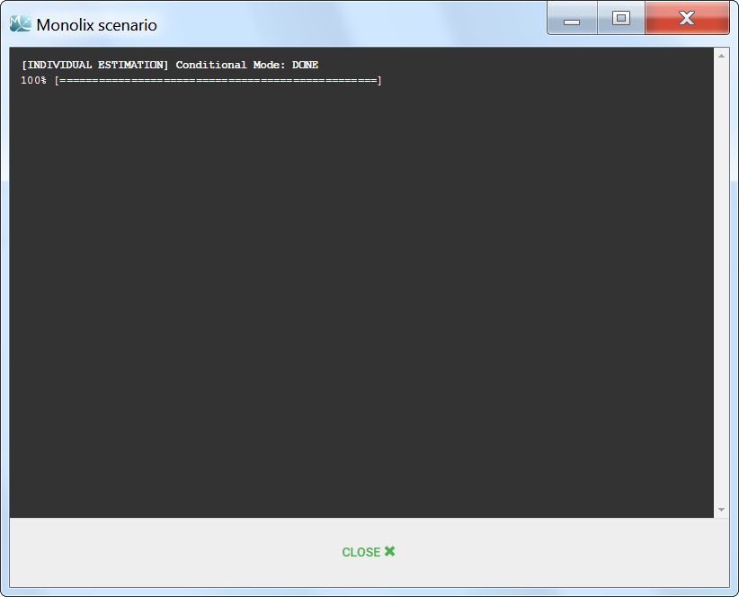
When running the EBEs task, the progress is displayed in the pop-up window:
Dependencies between tasks:
- The “Population parameters” task must be run before launching the EBEs task.
- The EBEs task is recommended before calculating the Standard errors task and the Log-likelihood task using the linearization method.
Outputs
In the graphical user interface
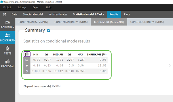
In the Indiv.Param section of the Results tab, a summary of the individual parameters is proposed (min, max, median, quartiles, and shrinkage [in Monolix 2024 and later]) as shown in the figure below. The elapsed time for this task is also shown.
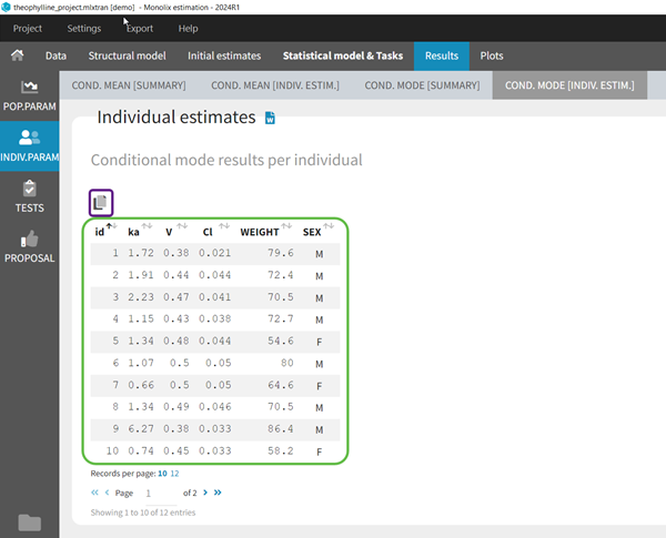
To see the estimated parameter value for each individual, the user can click on the [INDIV. ESTIM.] section. Notice that the user can also see them in the output files, which can be accessed via the folder icon at the bottom left. Notice that there is a “Copy table” icon on the top of each table to copy them in Excel, Word, … The table format and display will be kept.
In the output folder
After having run the EBEs task, the following files are available:
- summary.txt: contains the summary statistics (as displayed in the GUI).
- IndividualParameters/estimatedIndividualParameters.txt: the individual parameters for each subject-occasion are displayed. In addition to the already present approximation conditional mean from SAEM (*_SAEM), the conditional mode (*_mode) is added to the file.
- IndividualParameters/estimatedRandomEffects.txt: the individual random effects for each subject-occasion are displayed (*_mode), in addition to the already present value based on the approximate conditional mean from SAEM (*_SAEM).
- IndividualParameters/shrinkage.txt: starting with Monolix 2024, the shrinkage for each parameter for the conditional mode as shrinkage_mode.
More details about the content of the output files can be found here.
Settings
The settings are accessible through the interface via the button next to the EBEs task.
![]()
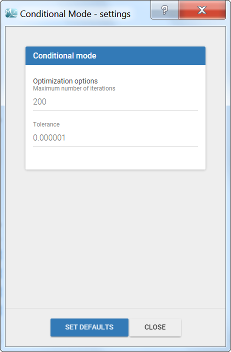
- Maximum number of iterations (default: 200): maximum number of iterations for the Nelder-Mead Simplex algorithm, for each individual. Even if the tolerance criteria is not met, the algorithm stops after that number of iterations.
- Tolerance (default: 1e-6): absolute tolerance criteria. The algorithm stops when the change of the conditional probability value between two iterations is less than the tolerance.