Purpose
This figure can be used to compare:
- the empirical distribution of the individual parameters, estimated with the conditional means, the conditional modes, or simulated from the conditional distributions,
- the theoretical distribution defined in the statistical model, with the estimated population parameter.
Further analysis such as stratification by covariate or shrinkage assessment can be performed and will be detailed below.
PDF and CDF
In the warfarinPK_project, several parameters are estimated. It is possible to display the theoretical distribution and the histogram of the empirical distribution as proposed below.
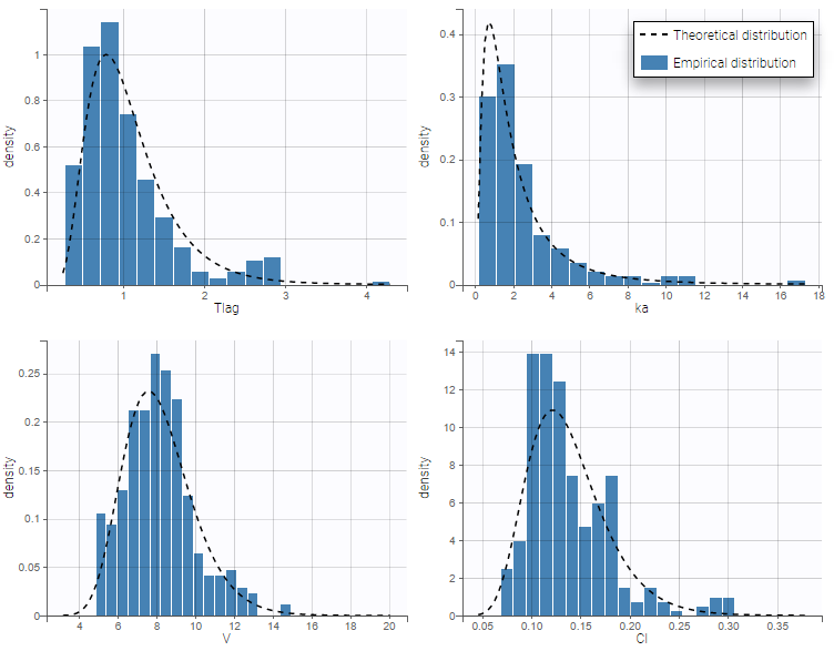
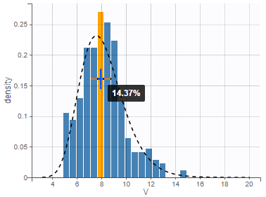
The distributions are represented as histograms for the probability density function (PDF). Hovering on the histogram also reveals the density value of each bin as shown on the figure below
Notice that the theoretical pdf is a pure log-normal distribution. However, in case of covariate use with the parameters, it is not a pure log-normal but rather a combinaison of log-normal distribution. If for example, on set the SEX covariate on the parameter V, a parameter beta_V_SEX_1 is created and the individual parameter distribution becomes as the following.
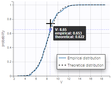
Cumulative distribution functions (CDF) is proposed too.
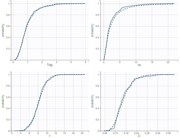
Again, overlaying the plots display the information concerning the parameter value and its empirical and theoretical cdf.
Getting away with shrinkage using simulated individual parameters
If the data does not contain enough information to correctly estimate some individual parameters, the individual estimates coming from the means or the modes of the individual conditional distributions shrink towards the same population value (respectively the mean or the mode of the population distribution of the parameter), a phenomenon known as shrinkage. For a parameter \(\psi_i\) that is a function of a random effect \(\eta_i\), this phenomenon can be quantified by defining the \(\eta\)-shrinkage as:
$$\eta\text{-shrinkage} = 1 -\frac{sd(\hat{\eta_i})}{\hat{\omega}} $$
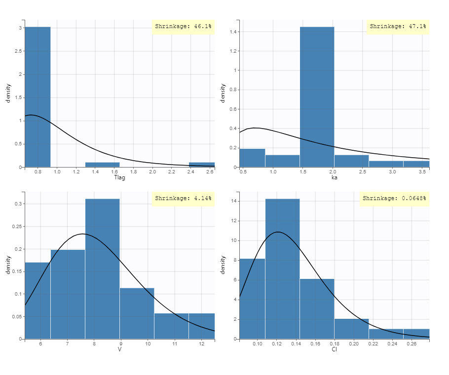
where \(\text{sd}\left(\hat{\eta}_i\right)\) is the empirical standard deviation of the estimated random effects \(\hat{\eta}_i\)’s. The \(\hat{\eta}_i\) can be calculated from the EBEs, the conditional mean or the samples from the conditional distribution. Typically, the shrinkage is reported using the EBEs. Previously, in Monolix version 2023 and earlier, shrinkage was defined based on the variance as \(\eta\text{-shrinkage} = 1 -\frac{Var(\hat{\eta_i})}{\hat{\omega^2}}\). It is possible to display the shrinkage value on top of the histograms, as seen below for the conditional mode (EBEs):
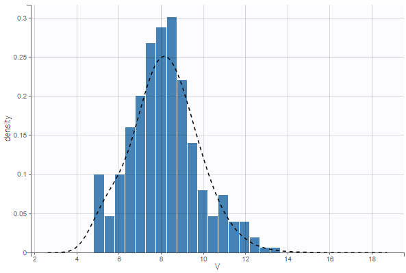
Selecting the “Conditional distribution” option instead for the individual estimates uses individual parameters drawn from the conditional distribution, simulated using MCMC sampling. This method is recommended as it results in unbiased estimators that are not affected by possible shrinkage, and leads to more reliable results. For more details see the page Understanding shrinkage and how to circumvent it.
In the same example, using the conditional distribution instead of the conditional mode reduces shrinkage, as can be seen below.
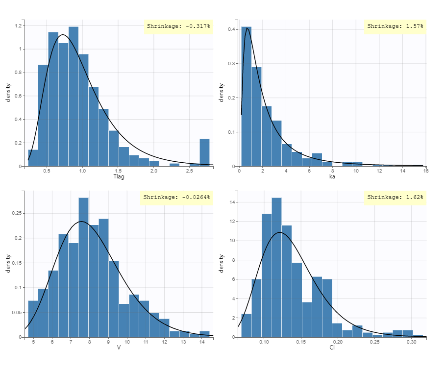
The following table shows the shrinkage calculation (in %) for all methods. The shrinkage is large for Tlag and ka when using the EBEs, which means that the individual data is not reach enough to reliable estimate the EBEs for Tlag and ka. The close to zero shrinkage value when using the samples from the conditional distribution shows that the samples from the conditional distributino are well spead over the population distribution, as expected.
| Method\Parameters | Tlag | ka | V | Cl |
|---|---|---|---|---|
| Conditional mean | 43.45 | 42.3 | 3.18 | 0.15 |
| Conditional mode (EBEs) | 46.07 | 47.11 | 4.14 | 0.065 |
| Conditional distribution | -0.317 | 1.57 | -0.26 | 162 |
Example of stratification
It is possible to stratify the population by some covariate values and obtain the distributions of the individual parameters in each group. This can be useful to check covariate effect, in particular when the distribution of a parameter exhibits two or more peaks for the whole population. On the following example, the distribution of the parameter k from the same example as above has been split for two groups of individuals according to the value of the continuous covariate AGE, allowing to visualize two clearly different distributions.

Settings
- General: add/remove the legend, the grid, and the shrinkage in %.
- Display
- Empirical: add/remove histogram of empirical distribution.
- Theoretical: add/remove curve of theoretical distribution.
- Distribution function: The user can choose to display either the probability density function (PDF) as histogram or the cumulative distribution function (CDF).
- Individual estimates: The user can define which estimator is used for the definition of the individual parameters.
Simulated individual parameters are used by default, otherwise the conditional mode is the default estimation if it has been computed with the “Individual parameters estimation” task.