- Purpose
- Calculation of the standard errors
- Running the standard errors task
- Outputs
- In the graphical user interface
- In the output folder
- Interpreting the correlation matrix of the estimates
- Settings
- Good practice
Purpose
The standard errors represent the uncertainty of the estimated population parameters. In Monolix, they are calculated via the estimation of the Fisher Information Matrix. They can for instance be used to calculate confidence intervals or detect model overparametrization.
Calculation of the standard errors
Several methods have been proposed to estimate the standard errors, such as bootstrapping or via the Fisher Information Matrix (FIM). In the Monolix GUI, the standard errors are estimated via the FIM. Bootstrapping can be accessed either through the Rsmlx R package or is now incorporated directly into the Monolix interface starting from version 2024R1.
The Fisher Information Matrix (FIM)
The observed Fisher information matrix (FIM) \(I \) is minus the second derivatives of the observed log-likelihood:
$$ I(\hat{\theta}) = -\frac{\partial^2}{\partial\theta^2}\log({\cal L}_y(\hat{\theta})) $$
The log-likelihood cannot be calculated in closed form and the same applies to the Fisher Information Matrix. Two different methods are available in Monolix for the calculation of the Fisher Information Matrix: by linearization or by stochastic approximation.
Via stochastic approximation
A stochastic approximation algorithm using a Markov chain Monte Carlo (MCMC) algorithm is implemented in Monolix for estimating the FIM. This method is extremely general
and can be used for many data and model types (continuous, categorical, time-to-event, mixtures, etc.).
Via linearization
This method can be applied for continuous data only. A continuous model can be written as:
$$\begin{array}{cl} y_{ij} &= f(t_{ij},z_i)+g(t_{ij},z_i)\epsilon_{ij} \\ z_i &= z_{pop}+\eta_i \end{array}$$
with \( y_{ij} \) the observations, f the prediction, g the error model, \( z_i\) the individual parameter value for individual i, \( z_{pop}\) the typical parameter value within the population and \(\eta_i\) the random effect.
Linearizing the model means using a Taylor expansion in order to approximate the observations \( y_{ij} \) by a normal distribution. In the formulation above, the appearance of the random variable \(\eta_i\) in the prediction f in a nonlinear way leads to a complex (non-normal) distribution for the observations \( y_{ij} \).
The Taylor expansion is done around the EBEs value, that we note \( z_i^{\textrm{mode}} \).
Standard errors
Once the Fisher Information Matrix has been obtained, the standard errors can be calculated as the square root of the diagonal elements of the inverse of the Fisher Information Matrix. The inverse of the FIM \(I(\hat{\theta})\) is the variance-covariance matrix \(C(\hat{\theta})\):
$$C(\hat{\theta})=I(\hat{\theta})^{-1}$$
The standard error for parameter \( \hat{\theta}_k \) can be calculated as:
$$\textrm{s.e}(\hat{\theta}_k)=\sqrt{\tilde{C}_{kk}(\hat{\theta})}$$
Note that in Monolix, the Fisher Information Matrix and variance-covariance matrix are calculated on the transformed normally distributed parameters. MonolixSuite version 2024R1 incorporates a change in the calculation of the variance covariance matrix \( \tilde{C} \). In version 2023 and before, \( \tilde{C} \) was obtained for untransformed parameters using the Jacobian matrix \(J\). The Jacobian matrix is a first-order approximation.
$$\tilde{C}=J^TC J$$
Starting from version 2024R1 and later, the Jacobian matrix has been replaced by exact formulas to compute the variance, dependent on the distribution of the parameters. Parameters are distingushed into those with normal distribution, lognormal distribution, as well as logit and probitnormal distribution:
- Normal distributed parameters: No transformation is required.
- Lognormal distributed parameters: The variance in the Gaussian domain (e.g variance of log(V_pop)) are obtained via the FIM. To obtain the variance of the untransformed parameyers (e.g variance of V_pop), the following formula is applied: \( Var(\hat{\theta}_{k}) = (\exp(\sigma ^{2}-1))\exp(2\mu + \sigma ^{2})\), with \( \mu = \ln(\hat{\theta}_{k}) \) and \( \sigma ^{2}=Var(\ln(\hat{\theta}_{k}))\)
- Logitnormal and probitnormal distributed parameters: There are no explicit formula to obtain the variance of the untransformed parameters (e.g bioavailability F) from the transformed parameter (e.g logit(F)). Therefore, a Monte Carlo sampling approach is used. 100000 samples are drawn from the covariance matrix in gaussian domain. Then the samples are transformed from gaussian to non-gaussian domain. For instance in the case of a logitnormal distributed parameter within bounds \( a\) and \( b\), the \(i\)-th sample of parameter \( \theta_{k,i}\): \(\mu_{k,i}=logit(\theta_{k,i})\) is transformed into non-gaussian space by the inverse logit, i.e. \(\theta_{k,i}=\frac{b \times \exp(\mu_{k,i})+ a}{(1 + \exp(\mu_{k,i}))}\). Then the empirical variance \(\sigma^2\) over all transformed samples \(\theta_{k}\) is calculated.
This transformation applies only to the typical values (fixed effects) “pop”. For the other parameters (standard deviation of the random effects “omega”, error model parameters, covariate effects “beta” and correlation parameters “corr”), we obtain directly the variance of these parameters from the FIM.
Correlation matrix
The correlation matrix is calculated from the variance-covariance matrix as:
$$\text{corr}(\theta_i,\theta_j)=\frac{\tilde{C}_{ij}}{\textrm{s.e}(\theta_i)\textrm{ s.e}(\theta_j)}$$
Wald test
For the beta parameters characterizing the influence of the covariates, the relative standard error can be used to perform a Wald test, testing if the estimated beta value is significantly different from zero.
Running the standard errors task
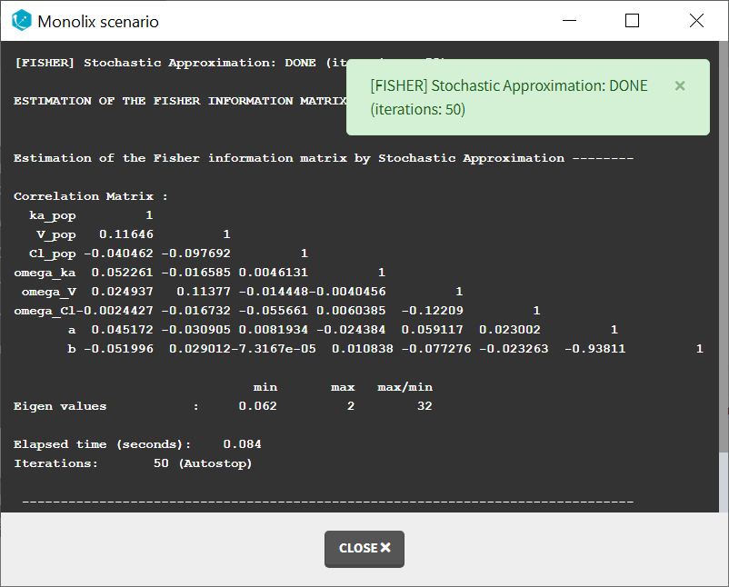
When running the standard error task, the progress is displayed in the pop-up window. At the end of the task, the correlation matrix is also shown, along with the elapsed time and number of iterations.
Dependencies between tasks:
The “Population parameters” task must be run before launching the Standard errors task. If the Conditional distribution task has already been run, the first iterations of the Standard errors (without linearization) will be very fast, as they will reuse the same draws as those obtained in the Conditional distribution task.
Output
In the graphical user interface
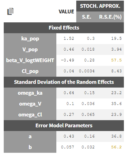
In the Pop.Param section of the Results tab, three additional columns appear in addition to the estimated population parameters:
- S.E: the estimated standard errors
- R.S.E: the relative standard error (standard error divided by the estimated parameter value)
To help the user in the interpretation, a color code is used for the p-value and the RSE:
- For the p-value: between .01 and .05, between .001 and .01, and less than .001.
- For the RSE: between 50% and 100%, between 100% and 200%, and more than 200%.
When the standard errors were estimated both with and without linearization, the S.E and R.S.E are displayed for both methods.
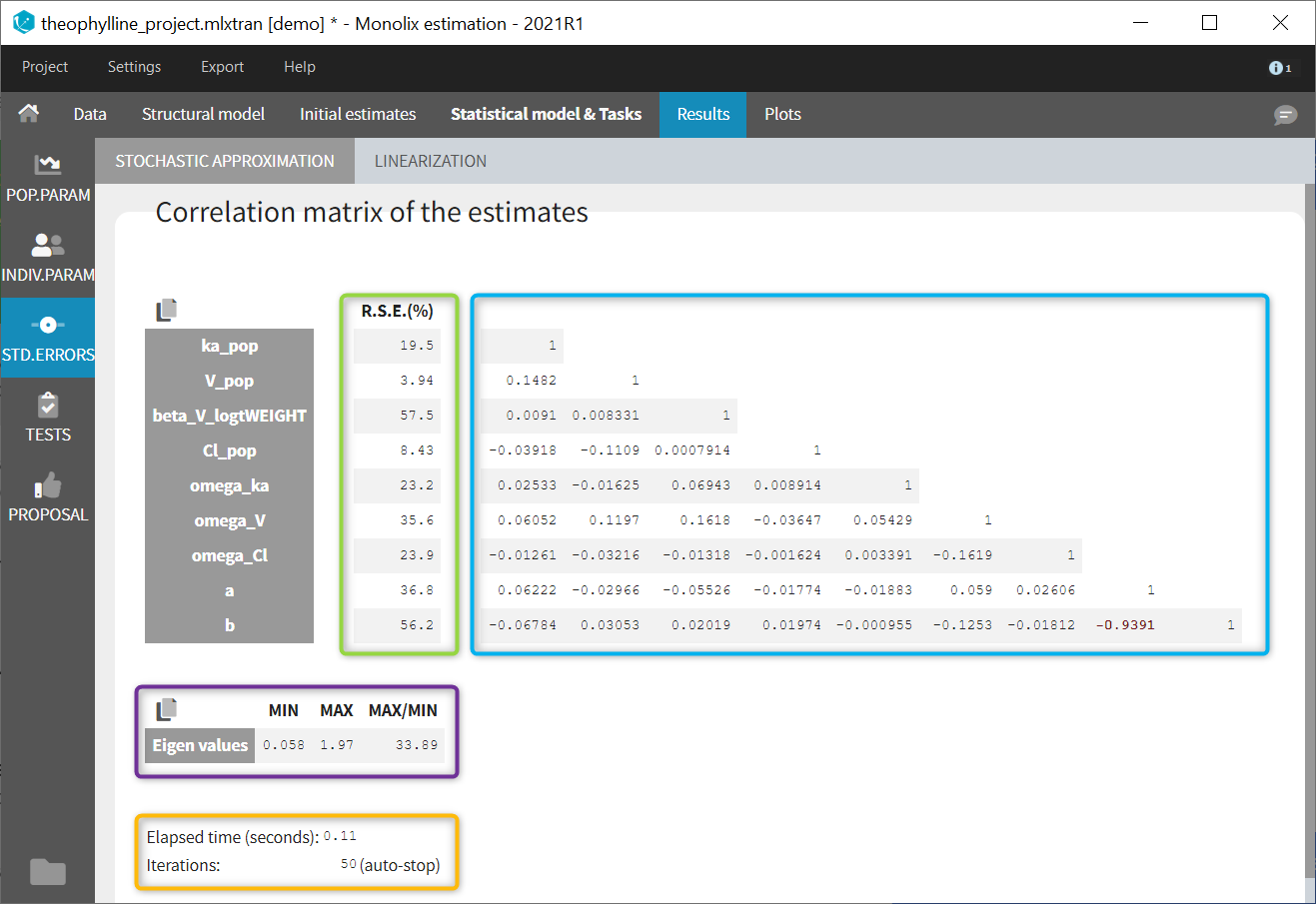
In the STD.ERRORS section of the Results tab, we display:
- R.S.E: the relative standard errors
- Correlation matrix: the correlation matrix of the population parameters
- Eigen values: the smallest and largest eigen values, as well as the condition number (max/min)
- The elapsed time and, starting from Monolix2021R1, the number of iterations for stochastic approximation, as well as a message indicating whether convergence has been reached (“auto-stop”) or if the task was stopped by the user or reached the maximum number of iterations.
To help the user in the interpretation, a color code is used:
- For the correlation: between .5 and .8, between .8 and .9, and higher than .9.
- For the RSE: between 50% and 100%, between 100% and 200%, and more than 200%.
When the standard errors were estimated both with and without linearization, both results appear in different subtabs.
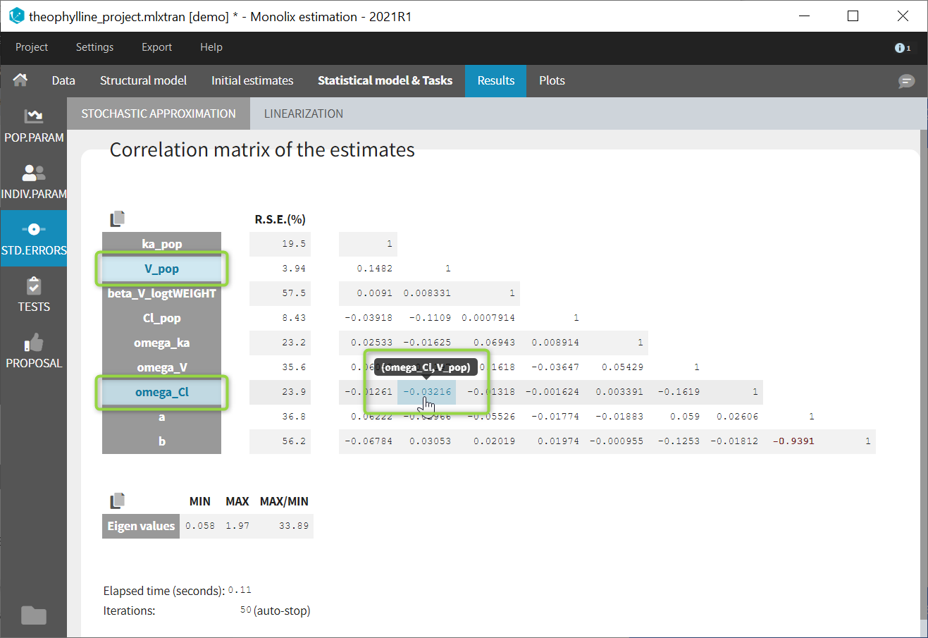
If you hover on a specific value with the mouse, both parameters are highlighted to know easily which parameter you are looking at:
In the output folder
After having run the Standard errors task, the following files are available:
- summary.txt: contains the s.e, r.s.e, p-values, correlation matrix and eigenvalues in an easily readable format, as well as elapsed time and number of iterations for stochastic approximation (starting from Monolix2021R1).
- populationParameters.txt: contains the s.e, r.s.e and p-values in csv format, for the method with (*_lin) or without (*_sa) linearization
- FisherInformation/correlationEstimatesSA.txt: correlation matrix of the population parameter estimates, method without linearization (stochastic approximation)
- FisherInformation/correlationEstimatesLin.txt: correlation matrix of the population parameter estimates, method with linearization
- FisherInformation/covarianceEstimatesSA.txt: variance-covariance matrix of the transformed normally distributed population parameter, method without linearization (stochastic approximation)
- FisherInformation/covarianceEstimatesLin.txt: variance-covariance matrix of the transformed normally distributed population parameter, method with linearization
Interpreting the correlation matrix of the estimates
The color code of Monolix’s results allows to quickly identify population parameter estimates that are strongly correlated. This often reflects model overparameterization and can be further investigated using Mlxplore and the convergence assessment. This is explained in details in this video:
Settings
The settings are accessible through the interface via the button next to the Standard errors task:

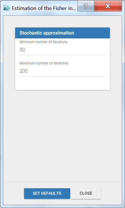
- Minimum number of iterations: minimum number of iterations of the stochastic approximation algorithm to calculate the Fisher Information Matrix.
- Maximum number of iterations: maximum number of iterations of the stochastic approximation algorithm to calculate the Fisher Information Matrix. The algorithm stops even if the stopping criteria are not met.
Good practices and tips
When to use “use linearization method”?
Firstly, it is only possible to use the linearization method for continuous data. For the linearization is available, this method is generally much faster than without linearization (i.e stochastic approximation) but less precise. The Fisher Information Matrix by model linearization will generally be able to identify the main features of the model. More precise– and time-consuming – estimation procedures such as stochastic approximation will have very limited impact in terms of decisions for these most obvious features. Precise results are required for the final runs where it becomes more important to rigorously defend decisions made to choose the final model and provide precise estimates and diagnosis plots.
I have NANs as results for standard errors for parameter estimates. What should I do? Does it impact the likelihood?
NaNs as standard errors often appear when the model is too complex and some parameters are unidentifiable. They can be seen as an infinitely large standard error.
The likelihood is not affected by NaNs in the standard errors. The estimated population parameters having a NaN as standard error are only very uncertain (infinitely large standard error and thus infinitely large confidence intervals).