Download data set only | Download all Monolix project files
Remifentanil is an opioid analgesic drug with a rapid onset and rapid recovery time. It is used for sedation as well as combined with other medications for use in general anesthesia. It is given in adults via continuous IV infusion, with doses that may be adjusted to age and weight of patients.This case-study shows how to use Monolix to build a population pharmacokinetic model for remifentanil in order to determine the influence of subject covariates on the individual parameters.
It is based on a data set of individual measurements, which was published in:
This data set is first explored with Datxplore. This allows to identify properties of the data set, leading to modeling hypotheses. Monolix is then used to quickly test these hypotheses implemented in a population pharmacokinetic model, evaluated with statistical tests and diagnostic plots.The data sets and the Datxplore and Monolix projects can be downloaded at the bottom of this page.
The case study is thus divided into several parts:
- Data set visualization with Datxplore
- Building a PK model using the library
- First evaluation: adjusting the structural model
- Second evaluation: adjusting the statistical model
- Final evaluation
- Conclusion
Data set visualization with Datxplore
65 healthy adults have received remifentanil IV infusion at a constant infusion rate between 1 and 8 µg.kg-1.min-1 for 4 to 20 minutes. The data set contains remifentanil administration characteristics (time and rate of infusion), with dense measurements of remifentanil plasma concentration during infusion and after (PK data). In addition, a several covariates are available: age, gender, and lean body mass (LBM). Moreover, a covariate TINFCAT classifies the patients in several categories with identical infusion duration.
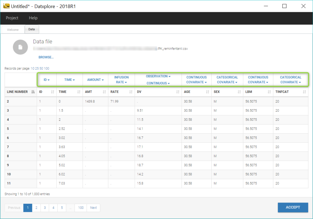
Below is an extract of the data set file:

Datxplore provides useful features to visualize the data and give indications about the structural model and the components of the statistical model. It also allows to identify potential covariates relationships and outliers.
We begin by opening the data in Datxplore (Menu: Project > New data). Datxplore infers the type of the columns which have standard names in the header (ID, TIME, AMT as AMOUNT, RATE as INFUSION RATE, DV as OBSERVATION, AGE as CONTINUOUS COVARIATE, SEX as CATEGORICAL COVARIATE). We set the other column types to CONTINUOUS COVARIATE for LBM and CATEGORICAL COVARIATE for TINFCAT.
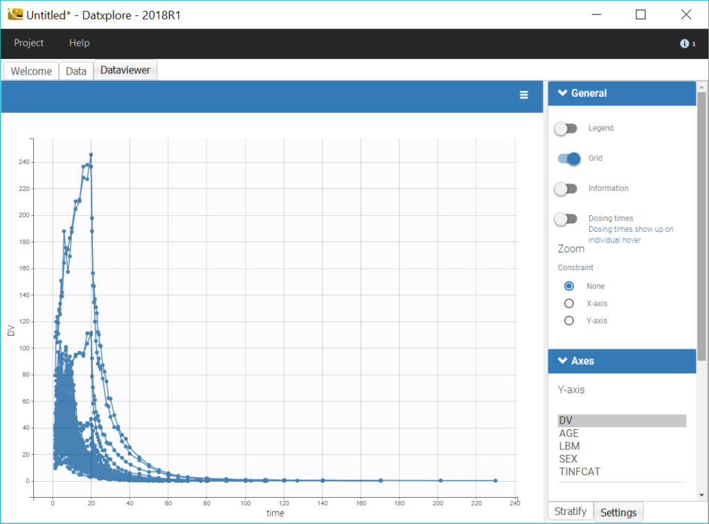
Datxplore automatically generates a number of plots to visualize the data. The spaghetti plot of the observations versus time is displayed below.
To reduce the heterogeneity in the plots, we split the data by infusion time category, by selecting TINFCAT in the Split panel and reordering the categories in four groups. In addition, using a log-scale for the y-axis is useful to identify kinetic properties.
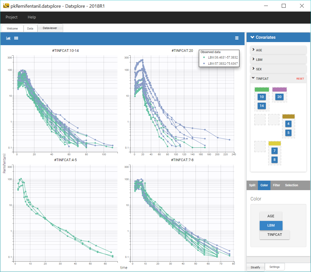
We can notice that the elimination of remifentanil in log-scale is non-linear just after the infusion, which suggests to use a PK model with several compartments, and linear for long times, which points toward a model with linear elimination.
Coloring the curves based on covariate values shows possible covariate effect, for example with LBM as shown on the figure above. Such covariate effect will be investigated further in Monolix later on.
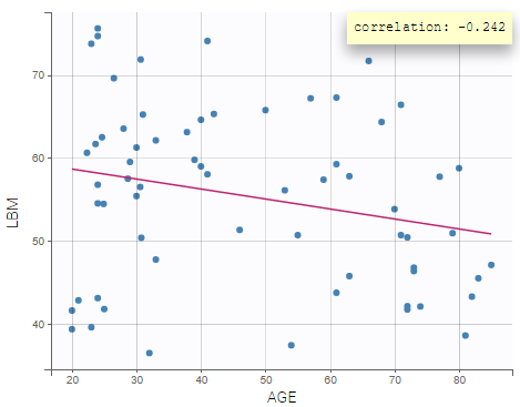
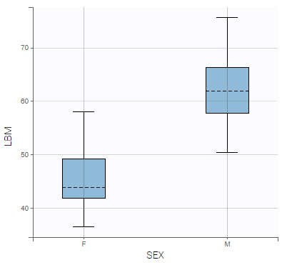
Correlations between covariates can also be identified, such as between LBM and AGE, and LBM and SEX:
 |
 |
|---|
In summary, from the data exploration in Datxplore, we have gained the following insights:
- A model with several compartments seems necessary to describe this dataset.
- LBM and AGE might have an effect on the pharmacokinetics
- LBM and AGE are negatively correlated, and males have higher LBM values than females.
We can then move to the model building process, while keeping in mind these properties that can guide the modelling process.
Building a PK model using the library
Defining the data
We open a new project in Monolix and we load the data PK_reminfentanil_data.csv (see download section) as previously done in Datxplore.
Defining the structural model: two compartments model with iv infusion and linear elimination.
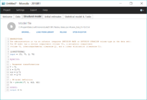
The next step is to define a structural model. As seen in Datxplore, we will first try an infusion model with two compartments and a linear elimination. This model is available in the Monolix PK library via “Load from library”: infusion_2cpt_ClV1QV2.txt.
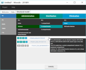
Once the model has been loaded, it is displayed on the interface, and can be opened in the editor. This model is written with the Mlxtran syntax using the macro pkmodel.
Selecting initial values
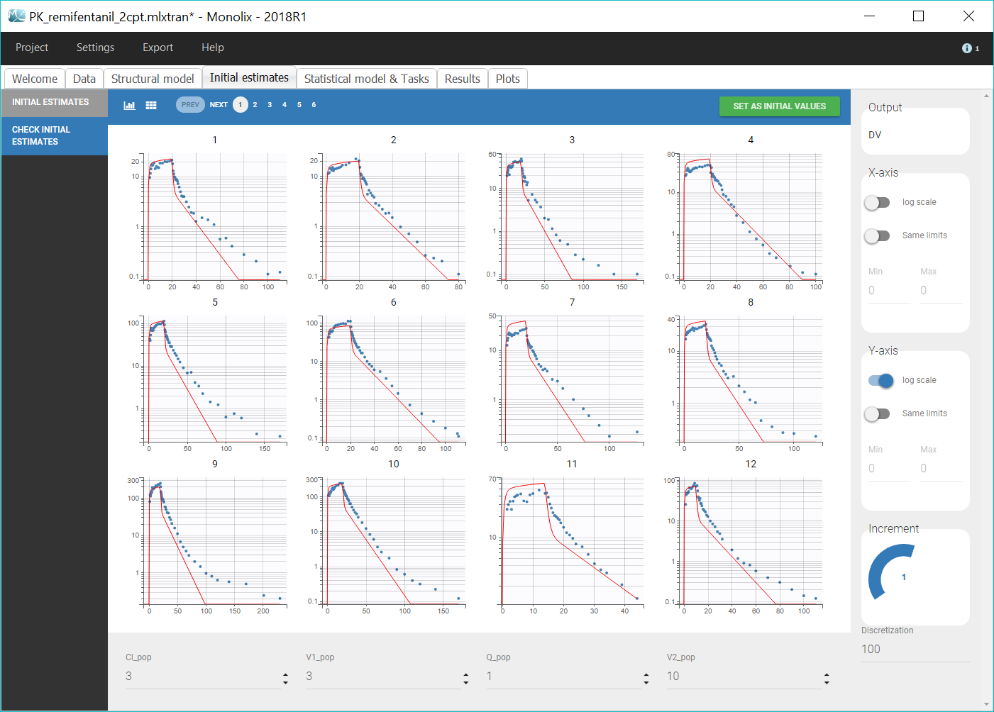
The next step is to select initial population parameter values in the “Initial estimates” tab. We can see the effect of the initial values on the prediction and how it fits the individual data on the “Check initial estimates” tab. The goal is to manually find population parameter values for which the prediction displays the key features of the model. For a 2-compartment model, this would mean seeing the two slopes in the elimination phase, on log-scale. Even if Monolix is pretty robust with respect to initial parameter values, it is good practice to choose reasonable initial estimates to speed up the convergence. We play with the values of the parameters until obtaining a reasonable agreement in both linear and log-scale, and we validate these values by clicking on “Set as initial values”. For example, as shown on the figure below, we can take Cl_pop=3, V1_pop=3, Q_pop=1 and V2_pop=10.
Defining the statistical model
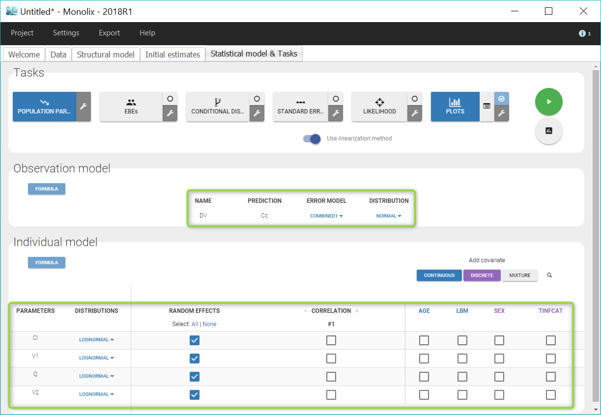
The “Statistical model & Tasks” tab can then be used to adjust the statistical model (green frames on the figure) as well as run estimation tasks. As a first step, we aim at evaluating the structural model, therefore we first keep the default statistical model: it is composed of a combined residual error model with an additive and a proportional term, and log-normal distributions for the individual parameters Cl, V1, Q and V2. We also ignore for now correlations between parameters or covariates.
First evaluation: adjusting the structural model
Once all the elements of the model have been specified, several tasks can be run in the “Statistical model & Tasks” tab to estimate the parameters and evaluate the model. It is important to save the project before (Project > Save), this way the result text files of all tasks run afterwards will be saved in a folder next to the project file. We save the project as PK_remifentanil_2cpt.mlxtran.
Several tasks can be run in a row by selecting all desired tasks and clicking on the green arrow (“Run scenario”), or tasks can be run one by one by clicking on each button. To evaluate quickly the structural model, we will keep the default scenario with only the population parameter estimation, and the diagnostic plots.
Estimating the population parameters
We first run the maximum likelihood estimation of the population parameters by clicking on “Population parameters”. This uses the stochastic approximation expectation-maximization (SAEM) algorithm. A pop-up opens where we can follow the estimation of the parameters over the algorithm iterations, and check the convergence.
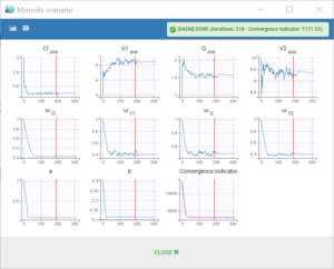
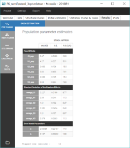
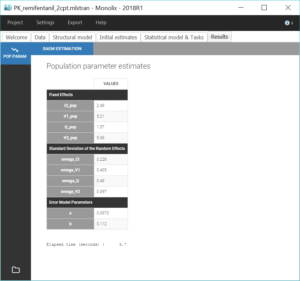
The estimated values can then be found in the tab “Results”.
Assessment of the structural model using the diagnostic plots
The last iterations of the SAEM algorithm are used to calculate a rough estimation of the individual parameters (conditional mean), which can be used for a first evaluation of the model without running the EBEs task. To assess the model, we run the task “Plots” to generate some diagnostic plots.
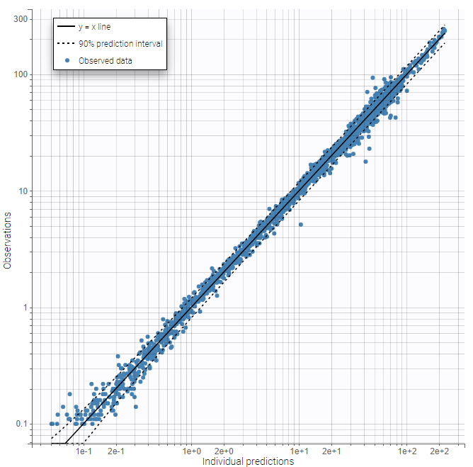
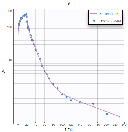
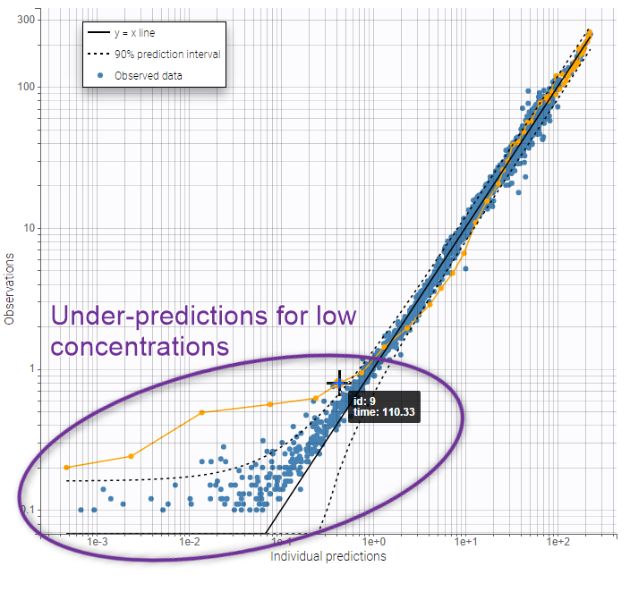
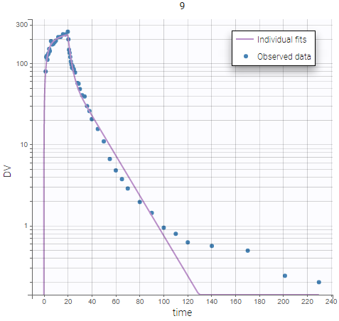
On the figures below we see first the Observations vs predictions plot, then an example of Individual fits plot. These plots show that low remifentanil concentrations are not well fitted: the two-compartments model seems unable to capture the different slopes of remifentanils elimination phase. This suggests to try a structural model with three compartments, in order to capture the three slopes that can be seen in the data.
 |
 |
|---|
Modifying the structural model: three-compartments model with IV infusion and linear elimination.
In the “Structural model” tab, we now load the model infusion_3cpt_ClV1Q2V2Q3V3.txt, which corresponds to a three-compartments model with IV infusion and linear elimination. We save the project in a new file PK_remifentanil_3cpt.mlxtran. As previously, we select reasonable initial values for the parameters (for example: Cl_pop=3, V1_pop=3, Q2_pop=1, V2_pop=10, Q3_pop=1, V3_pop=10) while keeping the default statistical model, and we run the population parameter estimation task as well diagnostic plots. We could also have used the option “use last estimates” in the “Initial estimates” tab in order to reuse the estimated parameters as starting point for the next run.
The same plots now show much better fits. We consider the 3 compartment model as our final structural model.
|
|
|
|---|
Further evaluation: adjusting the statistical model
Now that the structural model doe not show any mis-specification anymore, we can estimate individual parameters and assess the fit more precisely to evaluate improvements that might be brought to the statistical model.
Estimation of the individual parameters
We estimate the individual parameters with the task “EBEs”, which computes the mode of the conditional distribution for each individual, also called empirical Bayes estimates (EBEs). These values are the most likely parameters for each individual.
The next task, “Conditional distribution”, estimates each individual conditional distribution by sampling a set of values from the distribution via Markov Chains Monte Carlo. The results of this task increase the performance of model diagnostic plots, and avoid the phenomenon of shrinkage that can affect EBEs, in particular when the data is sparse.
In addition to the tab “Results”, the estimated individual parameters and individual random effects can also be found in table format in a new subfolder “IndividualParameters” in the project folder.
Estimation of the standard errors with the Fisher Information Matrix
We then compute standard errors for the population parameter estimates by clicking on the task “Standard errors”. This calculates the Fisher Information Matrix (FIM) via linearization of the model, or via stochastic approximation with the exact model if the option “use linearization method” is unchecked. The linearization method is faster and useful for large projects. Here we choose the stochastic approximation which is usually more precise. The standard errors and relative standard errors associated with each parameter can then be seen in the section “Pop. Param” of the tab “Results”, and the correlation matrix is displayed in the section “Std. errors”. We can check that all parameters have reasonable standard errors, meaning that all parameters are estimated with good confidence.
Estimation of the log-likelihood
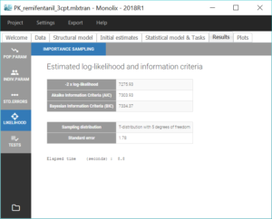
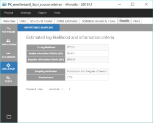
For the comparison of this model to more complex models later on, we can estimate the log-likelihood, either via linearization (faster) or via importance sampling (more precise). Clicking on “Likelihood” in the Tasks tab with the option “Use linearization method” unchecked, we obtain a -2*log-likelihood of 7255.32, printed in the “log likelihood” section of the “Results” tab, along with other information criteria (AIC and BIC):
Generation of the diagnostic plots
Finally, we run the plots again.
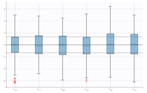
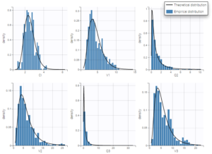
We check that there is no misspecification of the individual parameter distributions or the random effect distributions by looking at the plots Distribution of the individual parameters and Distribution of the standardized random effects (figures below). The first one shows the empirical distribution of the individual parameters as histograms overlayed with the theoretical parameter distribution. The second displays the standardized random effects plotted as boxplots. They are expected to follow a standard normal distribution, which is represented by the horizontal lines (median and quartiles).
 |
|
|---|
By default, these plots are based on the unbiased estimators sampled from the conditional distribution, rather than “Conditional mean” or “Conditional mode”, which cause -shrinkage. The plots shown above do not hint at any model mis-specification.
Moreover, p-values for Shapiro-Wilk normality tests in the section “Tests” on the “Results” tab could permit to detect misspecifications.
Adjusting the statistical model
Since the structural model is validated, we can use the estimated parameters as new initial values for the next run. This is done by clicking on the button “Use last estimates” in the “Initial estimates” tab. We can now adjust the statistical model.
Covariate search
Unexplained inter-individual variability may be reduced via the inclusion of covariates into the population PK model. Such effects can be suggested by correlations between covariate values and individual parameters, by looking at diagnostic plots and statistical tests in Monolix. In this case study, the workflow will be the following: we add covariates one-by-one, starting with the strongest significant correlation and checking at each step that the contribution to individual parameter variability is also significant. This stepwise manual method is suited to relatively simple models and allows the modeler to control each step of the model building process.
Interindividual variability explained by covariates can be identified on the plot Individual parameters vs covariates, where we notice correlations between some covariates and parameters. Note that Monolix uses samples from the conditional distribution to check correlation effects, a method that avoids the biases associated with conditional means or conditional modes (EBEs). Correlations can be displayed on the plots corresponding to continuous covariates using the “information” toggle in the settings.
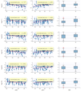
Additionally, the results of statistical tests checking correlation effects (Pearson correlation or ANOVA test for continuous or categorical covariates, respectively) are summarized in the section “Test” of the “Results” tab.
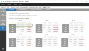
We start by adding the parameter-covariate relationship corresponding to the most significant p-value: it is the correlation between Cl and AGE. To obtain a power law relation between the parameter and the covariate, we first apply a centered log-normal transformation to the covariate AGE by clicking on “Add covariate: Continuous” in the “Individual model” section of the “Statistical model & tasks” tab. A pop-up window opens to define a new covariate with a formula. Hovering on AGE in this window gives its min, mean, median and max, which facilitates the centering. We define a new covariate tAGE = log(AGE/45.98).
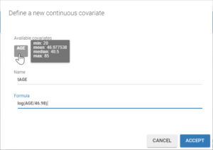
In the individual model, checking the corresponding box then sets a linear relation between log(Cl) and the new covariate tAGE displayed with a click on “Formula”. This relation involves a new individual parameter βCl_tAGE, that now has to be estimated.
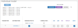
Before running, we save the project in a new file PK_remifentanil_3cpt_cov.mlxtran.
Assessment of the covariate model
To estimate the new parameter and assess the modified model, we run again the task scenario with 1) Population parameters estimation, 2) EBEs, 3) Conditional distribution, 4) Standard errors, 5) Plots.
The standard errors task also computes a Wald test on the individual estimates of βCl_tAGE to check that it is significantly different from 0, ie. that the relation between log(Cl) and tAGE is real. We obtain a p-value inferior to 1e-13, displayed in the “Population parameters” section of the “Results” tab:
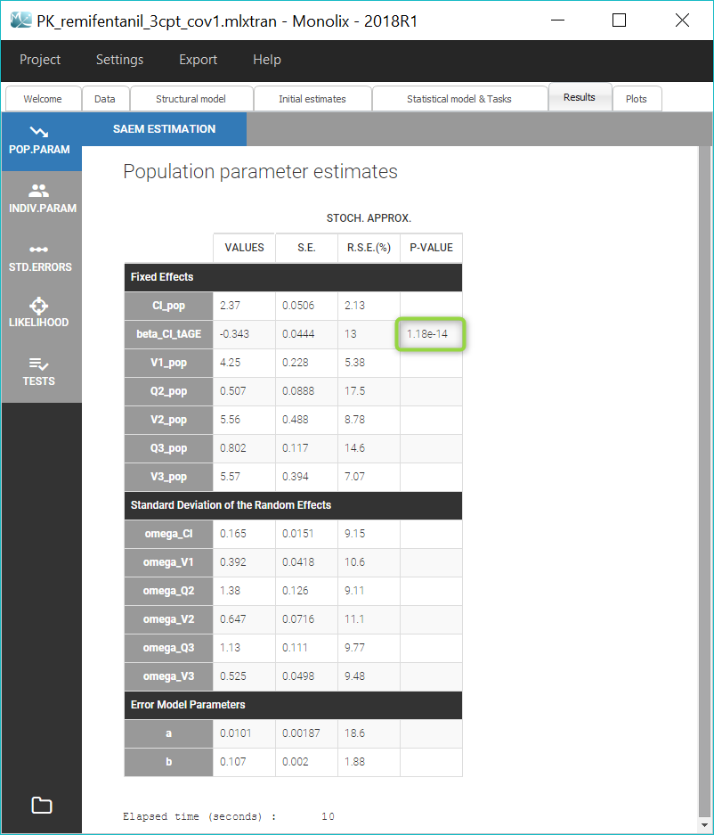
The details of the Wald test can also be found in the Tests part of the Results tab. Here we can also check that is no longer correlated with AGE (blue highlight below), because the correlation is taken into account in the model.
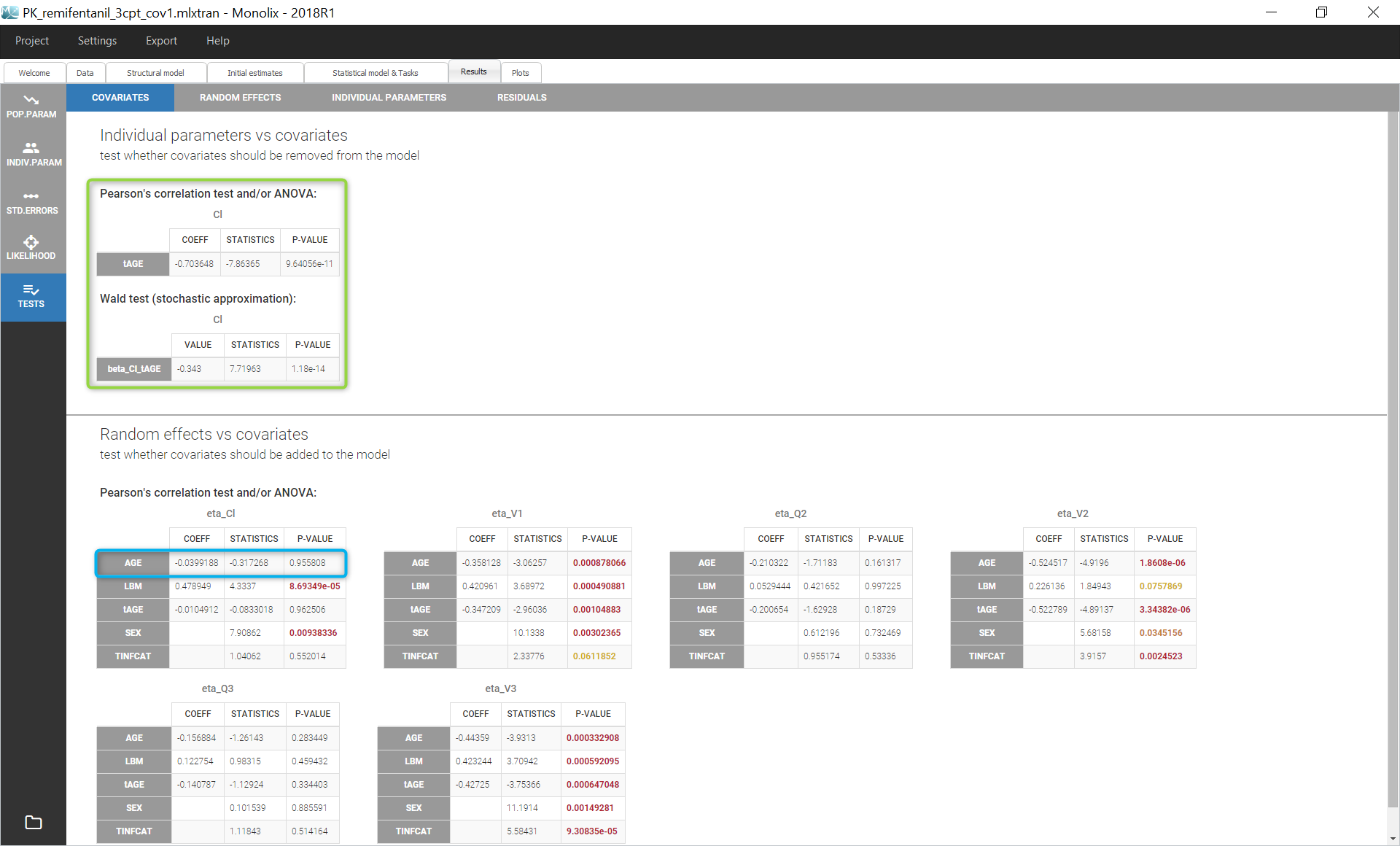
The small p-values validates the effect of AGE on Cl. We can then repeat the same procedure to add covariates to the model stepwise after setting the new estimates as initial values by clicking on the button “Use last estimates” in the “Initial estimates” tab.
The table below summarizes the successive steps in the covariate search, with the difference in AIC and BIC values between two successive runs. Note that the 8th model, in which AGE has been added on V1, results in higher values for AIC and BIC. Thus the effect of AGE on V1 does not bring improvement to the model and has to be removed. In addition, the p-value for the Wald test on βV1_tAGE at this step is 0.0353, confirming that AGE does not significantly explain variability in V1. The effect of V1 on AGE is then replaced by a weaker correlation that could be observed between AGE and Q2, which turns out to improve the model.
| Model name | Covariate effect | ΔAIC | ΔBIC | Keep the effect |
|---|---|---|---|---|
| model 1 | AGE on Cl | 41.73 | 39.55 | yes |
| model 2 | model 1 + AGE on V2 | 72.74 | 70.57 | yes |
| model 3 | model 2 + AGE on V3 | 38.45 | 36.27 | yes |
| model 4 | model 3 + LBM on V1 | 98.44 | 96.28 | yes |
| model 5 | model 4 + AGE on Q3 | 91.66 | 89.48 | yes |
| model 6 | model 5 + LBM on Cl | 26.33 | 24.05 | yes |
| model 7 | model 6 + LBM on V3 | 4.02 | 1.85 | yes |
| model 8 | model 7 + AGE on V1 | -1.07 | -3.24 | no |
| model 9 | model 7 + AGE on Q2 | 17.14 | 14.96 | yes |
The final covariate model includes tAGE on all parameters except V1, and the mean-centered log-transformation of LBM on Cl, V1 and V3. Correlations with the covariate SEX turn out to be all unsignificant: since SEX is also correlated to LBM, they are taken into account by the inclusion of LBM in the covariate model.
Correlations between random effects
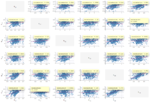
Correlations between individual parameters can be introduced in the model as linear correlations between the random effects, which are normally distributed random variables. Correlation effects can be identified for each pair of random effects with the p-values of Pearson correlation tests in the section “Tests” of the “Results” tab, and on “Correlations between random effects” plots, where correlation values can be displayed on scatter plots, as on the figure below.
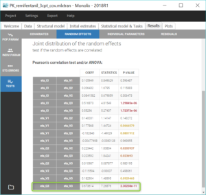
Similarly to the covariate search, we add relevant correlations to the model one-by-one, starting with the highest significant correlation (i.e lowest p-value), which is between Q3 and V3. After adding each correlation, we run the task scenario to update the scatter plots for pairs of random effects and the results of correlation tests, and we set the last estimates as new initial values for the estimation. The table below summarizes the three steps that allow to reach the final model, which is saved in the project PK_remifentanil_3cpt_covcor.mlxtran.
| Correlation between random effects | ΔAIC | ΔBIC |
|---|---|---|
| (Q3,V3) | 43.77 | 41.60 |
| (Q3,V3,Cl) | 38.12 | 33.77 |
| (Q3,V3,Cl) and (Q2,V2) | 4.9 | 2.72 |
The final model includes a correlation between Cl, Q3 and V3, and a correlation between Q2 and V2.

Running the log-likelihood task yields smaller values for the information criteria than previously (ΔAIC=477.2 and ΔBIC=451.1 compared to PK_remifentanil_3cpt.mlxtran): the difference in each criterion indicates the improvement of the model through covariates and correlations effects.
Assessing the error model
While looking at the estimated population parameters in the section “Pop. Parameters” of the tab “Results”, we notice that the estimate a_pop for the constant residual error is low compared to the concentration data (a=0.003 versus concentration data range=0.1-300). This leads us to try a simpler observation model with a proportional residual error.

After executing the whole task scenario, this choice results in a very close although higher value for AIC (ΔAIC=2.01). Therefore the proportional error model seems sufficient.
Final evaluation
Visual Predictive Check
To perform a final evaluation of our model, we generate the Visual Predictive Check by selecting the VPC option in the list of plots before running the task.


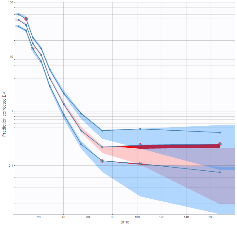
The VPC is based on multiple simulations with the model and the design structure of the observed data, grouped in bins over successive time intervals. It is a useful tool to assess graphically whether simulations from the model are able to reproduce both the central trend and variability in the observed data. It is fast to generate in spite of the big number of simulations (500 by default). The median and percentiles of the observed data are plotted in blue curves and can be compared to the corresponding prediction intervals: areas in blue and pink respectively. Discrepancies are highlighted in red.
Selecting corrected predictions in “Settings” takes into account the high heterogeneity in doses. The result, on the figure below wiht log-scale on the Y-axis and 10 bins, is satisfying. From the discrepancy seen at low doses, we may hypothesize that BLQ data have been observed but were excluded from the data set.
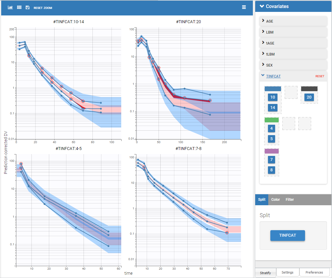
Splitting the plot according to the categorical covariate “TINFCAT” in “Stratify” allows us to better see the predictions for more homogeneous subpopulations, including the absorption phase when the data is sufficient, as seen on the figure below. The remaining discrepancies affect mainly the subplot corresponding to TINFCAT=20, which is the group with the most variability in the dataset.
Convergence Assessment
Finally, we can check that the convergence and the estimates are robust to different initial estimates.
The convergence assessment tool, launched with the grey button just below the green arrow in the task tab, executes multiple runs of parameter estimation and model evaluation with different seeds and random initial values of fixed effects. It returns a graphical report that allows to compare the convergence of the parameter estimation and the estimates between runs.
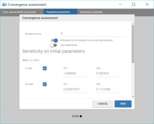
Clicking on the assessment task first opens a window where we can choose the number of runs used for the assessment, the tasks performed during each run, and the parameters checked for sensitivity. Here we choose to estimate the standard errors and log-likelihood without linearization to get precise results, over 5 replicates, with randomly picked initial values for all parameters.
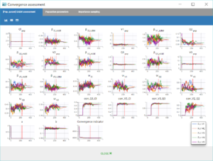
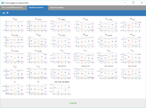
The displayed figures show a good convergence of all replicates to the same minimum.
Conclusion
In this case-study, Monolix has been used to easily build a population model for remifentanils pharmacokinetics. Each step of model modification was guided by diagnostic plots and statistical tests to check the accurateness of the model and its properties. This process allowed a manual covariate search that revealed a dependency of several parameters on the age or the lean body mass.
This model could now be imported with the R package Simulx to be simulated, either with its initial dataset or with new specifications: different treatments, number of subjects, covariates… Examples of applications include clinical trial simulations to determine the best dosing protocol, or assessing the uncertainty of the results according to the number of individuals.
