This case study uses the MonolixSuite to analyze and model the absorption and elimination of alcohol with or without a dietary additive of guar gum. It focuses in particular on the modeling of inter-occasion variability.
Guar gum, also called guaran, is a polysaccharide extracted from guar beans. As a natural polymer, it has been used for many years as an emulsifier, thickener, and stabilizer in the food industry. In the pharmaceutical sector, guar gum and guar-gum based systems are frequently studied for the development of controlled-released formulations and colon targeted drug delivery systems, as guar gum can protect active molecules from the enzymes and pH in the stomach and small intestine and it can be degraded by intestinal bacteria in the colon. [Aminabhavi, T. M., Nadagouda, M. N., Joshi, S. D., & More, U. A. (2014). Guar gum as platform for the oral controlled release of therapeutics. Expert Opinion on Drug Delivery, 11(5), 753–766.]
Moreover, guar gum may affect the bioavailability of concomitantly administered substances due to its effect on the rate of gastrointestinal transit and gastric emptying.
The goal of this case study is then to assess the effect of guar gum on the absorption and bioavailability of alcohol.
Outline:
Data set
The data has been published in:
Practical Longitudinal Data Analysis, David J. Hand, Martin J. Crowder, Chapman and Hall/CRC, Published March 1, 1996
It is composed of measurements of blood alcohol concentrations in 7 healthy individuals. All subjects took alcohol at time 0 and gave a blood sample at 14 times over a period of 5 hours. The whole procedure was repeated at a later date but with a dietary additive of guar gum. The two different periods of time are encoded in the data with overlapping times, both starting at time 0.
Although the precise amount of ingested alcohol is unknown, for this case study we assume each amount to be 10g (standard drink).
Data exploration in Datxplore

The data is loaded in Datxplore to explore it graphically. It appears in the Data tab as above. The time is in hours, the alcohol concentration in the column Y is in mg/L, and the amount in AMT is in mg. Censored observations are indicated with the column CENS tagged as CENSORING.
The two periods of measurements, during which the subjects have received or not guar gum in addition to alcohol are distinguished with the column OCC, which is automatically recognized as OCCASION. In addition, I use the column DIET that I tag as CATCOV to indicate which occasion corresponds to the addition of guargum. This column contains 2 strings: noGuar for occasion 1 and withGuar for occasion 2.
In the Plots tab, the plot of alcohol concentration vs time in log-scale seen below suggests to use a one-compartment model with a first-order absorption. A non-linear elimination appears for some individuals, but the data might not be sufficient to capture it. Thus a linear elimination should be tried as a first model.
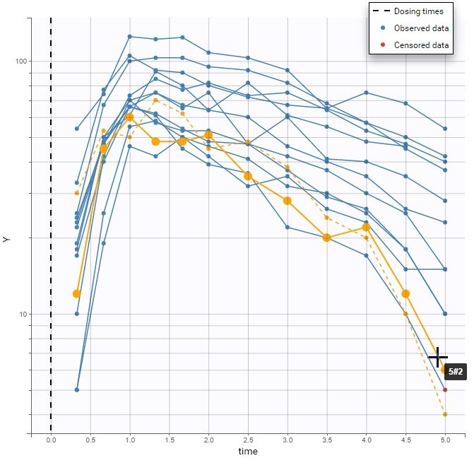
The different occasions can be visualized in several ways. First, hovering on a curve highlights the curve in solid yellow and the curve corresponding to the other occasion from the same subject in dashed yellow, as on the figure above.
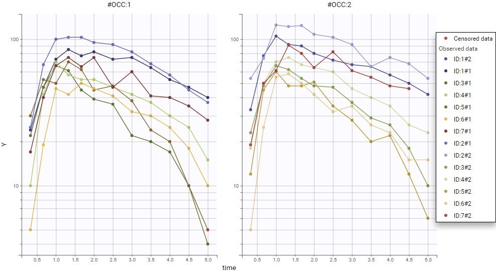
Second, OCC is available for stratification along with the covariate DIET in the “Stratify” panel , and can thus be used for splitting, coloring or filterting. Below are for example the subplots of the data split by OCC and colored by ID. Each subject-occasion is assigned a color, with matched color shades for subject-occasions corresponding to the same subject. This is convenient to compare at a glance the two occasions for all subjects. The inter-individual variability seems mostly reproduced from one occasion to the other, and concentration levels seem slightly higher for OCC=2.
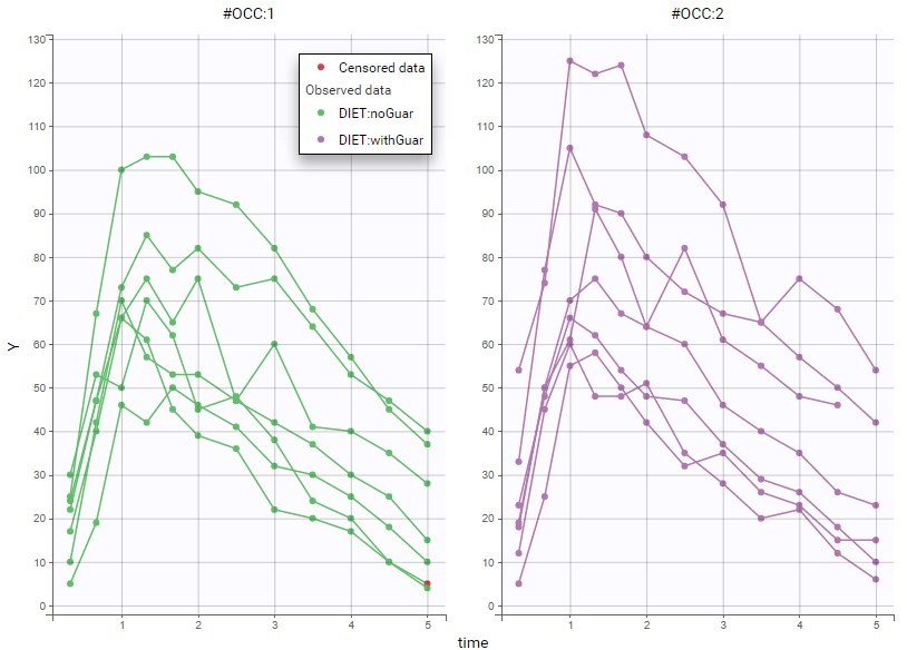
This global trend can be confirmed in linear scale below. Here the plot is colored by DIET, whose categories are matched with OCC: DIET=noGuar corresponds to OCC=1 and DIET=withGear to OCC=2. Thus, the main inter-occasion variability seen in the data seems to be explained by the covariate DIET.
First analysis in PKanalix
Non-compartmental analysis
As a first analysis, we can check the difference in PK parameters for the two occasions with non-compartmental analysis (NCA) in PKanalix. After loading the previously saved Datxplore project in PKanalix, the following settings are chosen:
- extravascular administration,
- “linear up log down” integral method,
- “missing” for blq after Tmax (censored observations after Tmax are not used in the analysis).
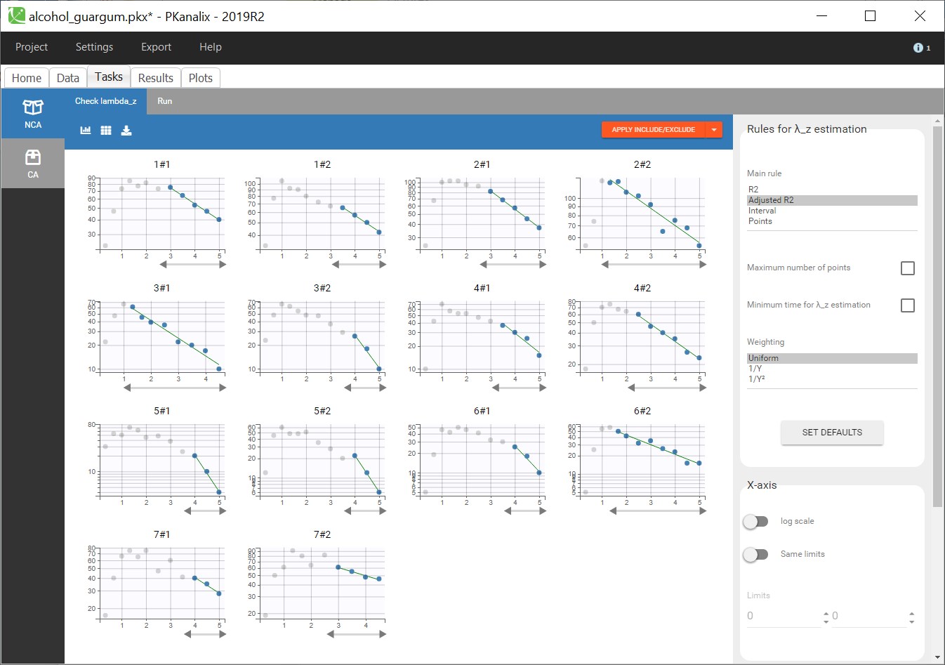
The “Check lambda_z” panel, seen below, allows to check the regressions estimating the elimination slope. The default “adjusted R2” rule selects for each individual the optimal number of points used in the regression to get the best regression. While the plots allow to adjust the selection of points for some individuals, it is not necessary here. The plots already show some variability between individuals in the estimated lambza_z.
Running the NCA gives the lambda_z and other PK parameters for each individual. In the “Plot” tab, the plot of individual parameters vs. covariates is convenient to visualize the variability in the parameters and compare the distributions without and with guar gum. Here the following parameters have been selected: AUCINF_pred, Cl_F_pred, Cmax, HL_Lambda_z, Tmax:
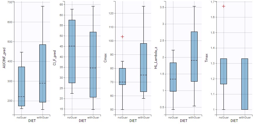
Some difference can be seen between the two conditions for the half-life, the apparent clearance and Cmax, however the parameters also show large variability within each dietary condition.
Compartmental analysis in PKanalix
Next, a compartmental analysis (CA) can be run to estimate a compartmental model and compare the estimated parameters between the two conditions. PKanalix considers that the subject-occasions are independent, thus the parameters are optimized independently on each individual and on each occasion. This allows to check easily if different values are estimated for the two occasions.
Choosing a one-compartment model with a first-order absorption and a linear elimination gives the following individual fits (after choosing initial values with the “aut-init” button):
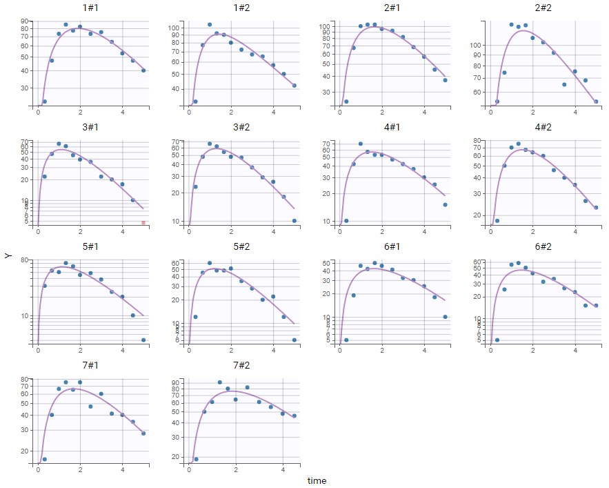
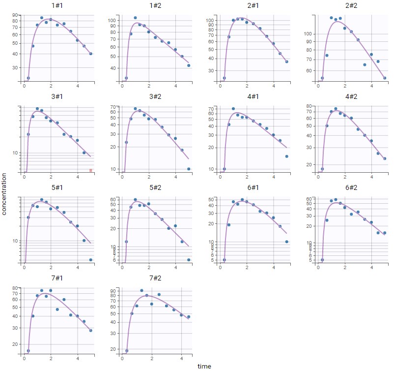
The absorption phase is not really well captured. Zooming on this phase can help confirm that the absorption should be delayed. Choosing the same model as before but with a lag time before the absorption now gives good individual fits:
 In the plot Individual parameters vs. covariates, the estimated individual parameters show different distributions across the two conditions of DIET, in particular for ka, V and k:
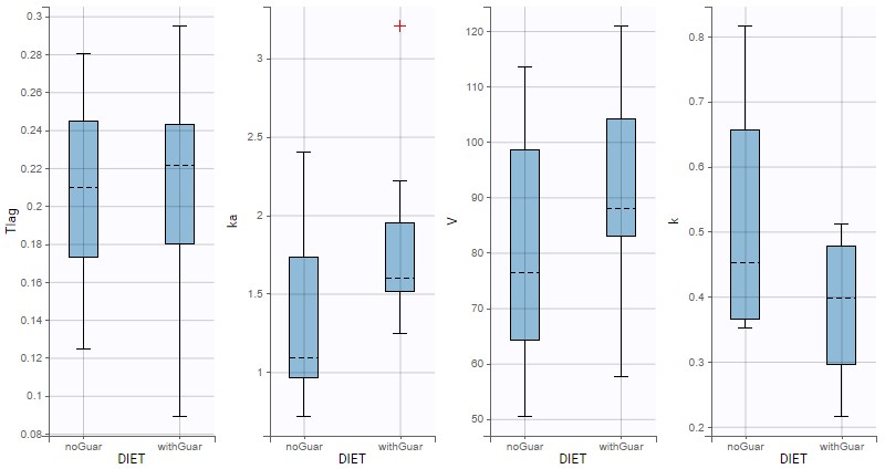
Since the data size is small, it is not clear whether these differences are significant. The effect of DIET on the alcohol kinetics can be assessed more precisely with a detailed population analysis in Monolix.
Moreover, the bioavailability is not explicitly taken into account by this model, because it is not identifiable with only extravascular administrations, so it is included in the apparent volume V. In Monolix, it is possible to use more complex models than the simple PK models from the library, and in particular to add the bioavailability explicitly, allowing to assess in a more meaningful way whether guar gum could have an effect on the relative bioavailability depending on the value of DIET.
Therefore, we export the compartmental model from PKanalix to Monolix.
Population modelling in Monolix
This opens a Monolix project in which the data and the structural model are set up like in PKanalix.
In “Statistical model & Tasks”, the “Individual model” part is now split in two. The part on the left at the ID level describes the inter-individual variability (IIV), and includes by default a random effect for each parameter. The part on the right (highlighted in the figure below) is dedicated to the OCC variability-level, where it is possible to add random effects at the inter-occasion level: this would create inter-occasion variability (IOV). Since DIET varies from one occasion to another, it appears in this panel to explain part of the inter-occasion variability with a covariate effect. The boxes for adding covariate effects are greyed out, because at this step there is no inter-occasion variability. It is only possible to add covariate effects at the occasion level on parameters that either have inter-occasion variability with random effects at the occasion level, or parameters that have no random effects at the id and occasion levels.

Model without inter-occasion variability
The first step in this worklow aims at validating the structural model without taking into account differences between the occasions. Thus we keep the statistical model to default, select all tasks in the scenario and save the project as run01.mlxtran.
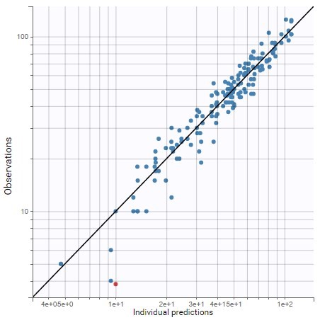
Estimating this model does not show misspecifications on the plot of Observations vs Predictions in log-log scale:
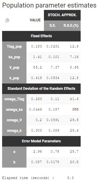
All parameters are estimated with a good confidence, except omega_ka which is small and with a high rse:
On the individual fits seen below, disabling the option “Split occasions” in “Display” allows to visualize the two occasions on the same plot for each individual. The observed data can be colored by occasion or equivalently by DIET in Stratify.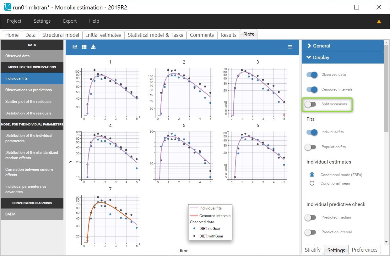
In this case, the predictions are identical for both occasions and overlap, since no inter-occasion variability is taken into account in the model. The prediction curves are displayed in purple for the first occasion and orange for the second, by default the curve for the first occasion on top, except for the last individual for which the second occasion is on top because it corresponds to a smaller observation period.
The individual fits shows that capturing both occasions with the same prediction is not possible, because there are small non-random variations from one occasion to another, as seen during the data exploration. This could corresponds to variability in the parameters between the occasions, that can be taken into account in the “Statistical model & Tasks” tab, by adding some random effects at the inter-occasion level or defining a covariate effect of DIET. We will first focus on the random effects.
Model with relative bioavailability and unexplained inter-occasion variability
Each parameter can be modelled with IIV, IOV or both. Physiological considerations can help deciding if a parameter should have variability at each level or not. But in the absence of clear physiological knowledge, a possible approach is also to add a random effect at the occasion level on each parameter for which variability may be relevant, and check if the estimated standard deviation of the random effect is small.
In this case, all parameters may show some inter-occasion variability. Indeed, the elimination can easily show some variations between different periods, and the dietary additive of guar gum might change the values of the parameters Tlag and ka characterizing the absorption. The volume V is unlikely to vary much for one occasion to another, however in this case V corresponds to the apparent volume, that includes the bioavailability of alcohol, which may vary with guar gum. Thus, it would be possible to set a random effect for IOV on V, or alternatively to modify the structural model to include explicitly the bioavailability, and add the random effect at the occasion level on the bioavailability instead of the volume. This is what we are going to do.
Before modifying the structural model, we use the last estimates as new initial values to facilitate the estimation for the next run.
Then, we open the structural model in the editor, and add an argument p=F in the pkmodel macro. This means that the proportion of absorbed drug will be defined by the parameter F, that should also be added in the input list:
[LONGITUDINAL]
input = {Tlag, ka, V, k, F}

EQUATION:
; PK model definition
Cc = pkmodel(Tlag, ka, V, k, p=F)

OUTPUT:
output = Cc
This modified model is then saved under a new name. The compile button is convenient to check that there is no syntax error. The new model can then be loaded in Monolix instead of the previous one.
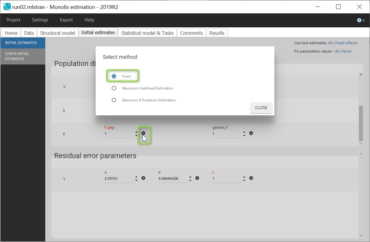
After loading the model, Monolix brings us to the “Check initial estimates” tab to choose a good initial value for F_pop. Here F is not the absolute bioavailability, but it corresponds to a relative bioavailability between the individuals. Thus F_pop is the reference value for the bioavailability, and it should be fixed to 1. This can be done in the list of the initial estimates, by changing the estimation method for F_pop to “Fixed”:
Now that the model includes the relative bioavailability explicitly, we can consider IOV for F instead of for V. Since V and F are not identifiable together, we should not include IIV for F while there is already IIV for V.
Clicking on Formula displays the model for the individual parameters. For instance, the model for Tlag now includes a random effect eta_OCC_Tlag in addition to the random effect eta_ID_Tlag:
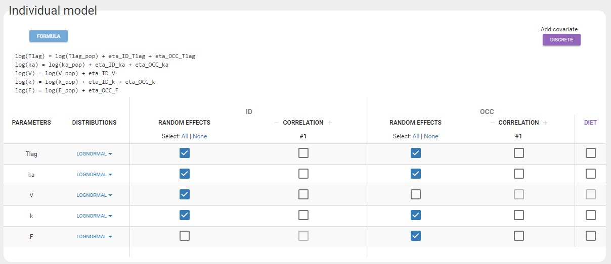
This project is saved as run02.mlxtran and all tasks are run.
The table of population parameters now include the standard deviations of the new random effects at the OCC level, which are called gamma:
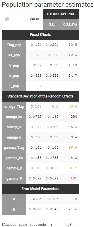
There a few high rses for the standard deviations of the random effects, because it is not possible to identify well all the random effects with such a small dataset. The random effects with the smallest standard deviations could probably be removed, such as omega_ka or gamma_F. In a later step, we will check more precisely which random effects should be removed. For now, we will first check the relationships between the random effects and the covariate DIET.
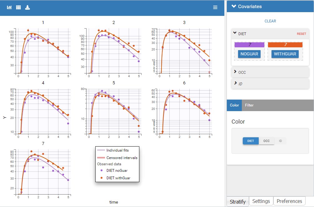
On the individual fits, there are now different individual predictions for each occasion. The colors associated to each value of DIET for the observations can be changed in “Stratify” to match the colors of the predictions. The predictions from occasion 1 are in purple, they correspond to the first category noGuar. The second category withGuar corresponds to the second occasion with orange predictions.
After clicking on Information, the individual parameter values appear on the plots for each occasion (for example here for the two first individuals):
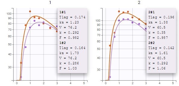
For V, which has only IIV, a single value is estimated for each individual across both occasions. For F, which has only IOV, it is important to note that estimated individual random effects from the distribution defined by gamma_F are independent across ids and occasions, and take into account the fact that F is slightly different for all subject-occasions. So a different value is estimated for each subject-occasion. Thus, the inter-occasion variability represents also an inter-individual variability. For parameters that have both IIV and IOV (Tlag, ka and k), the variability at the id level represents the additional variability between individuals that is common across both occasions.
The individual fits show that the IOV allows to properly capture the observations for each subject-occasion, and the predicted alcohol concentration seems usually higher when individuals have taken guar gum, except for ids 5 and 6. Let’s check this with the other diagnostic plots.
Assessing the effect of guar gum on alcohol’s PK
First, the plot of individual parameters vs covariates can be used to compare the distributions of each parameters across the two occasions.
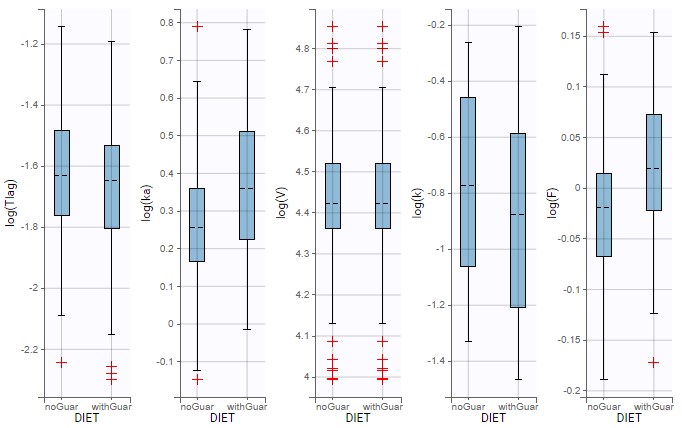
Notable differences appear for ka, k and F. The kinetics with guar gum exhibit higher absorption rates and bioavailability, and smaller elimination rates. We can try to implement one or several of these differences in the model with a covariate effect, starting with the hypothesis that guar gum could affect the bioavailability of alcohol.
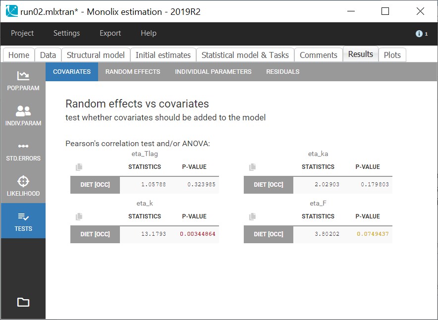
The statistical tests in Results show that these differences do not correspond to a significant correlation between eta_ka and DIET, but there is a significant correlation with eta_k, and a slightly significant correlation with eta_F. The lack of significance for ka and F is explained by the small size of the data which affects the p-values.
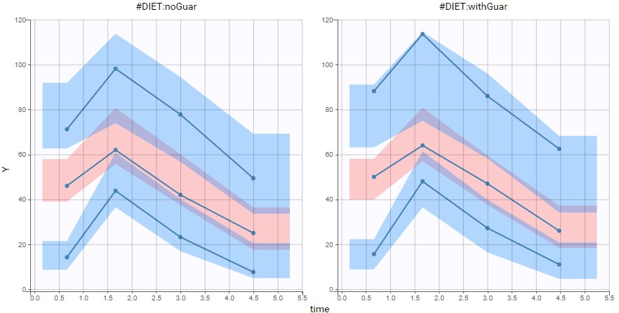
Second, we can have a look at the VPC split by DIET. Here, the prediction intervals are based on simulations that use the IOV included in the model, which is independent from DIET. Thus the prediction intervals are almost identical on each plot, while the empirical curves differ with DIET.
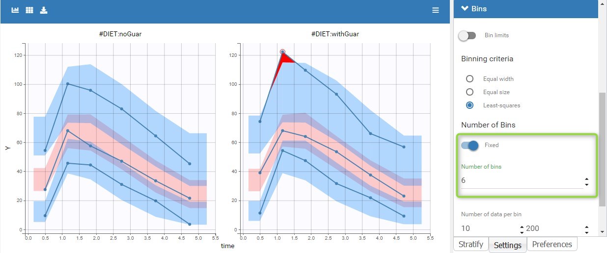
With the 4 bins computed by default, empirical curves are well captured by the prediction intervals, so with this size of data, the small differences caused by guar gum do not cause a visible discrepancy of the model, but when setting the number of bins to 6 (see below), a small discrepancy appears in the absorption phase. Although we should keep in mind that the empirical percentiles represent only a small number of individuals, this is a hint that it could be relevant to take into account an effect of guar gum on the absorption or the bioavailability.
Model with inter-occasion variability and occasion-varying covariate effect
As a result of this diagnosis, we can now adjust the model, after using the last estimates as new initial values. Based on the diagnostic plots and the biological knowledge on possible mechanisms for the effect of guar gum, we will try to explain part of the IOV by adding a covariate effect of DIET on F. We save this modified project as run03.mlxtran and run all tasks.
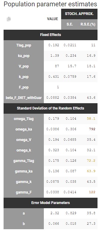
The new parameter beta_F_DIET_withGuar is estimated to a small value (0.08) but with a good standard error, and it results in a small decrease of gamma_F (from 0.07 to 0.034):
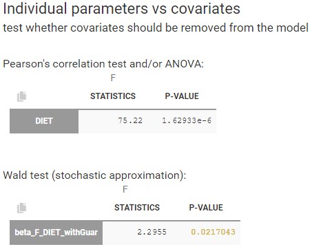
In the statistical tests, the p-value for the Wald test, which checks whether the parameter is close to 0, is small but the test is not quite significant. In addition, the correlation between F and DIET is significant:
The diagnostic plot also show that this correlation is strong: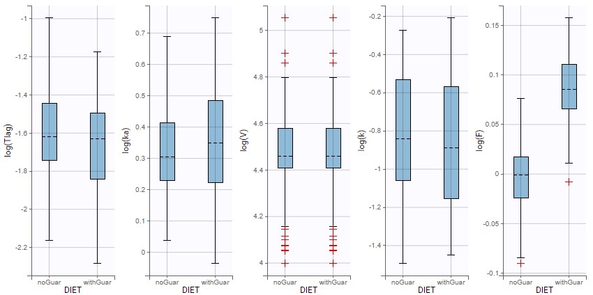
Therefore the covariate effect is relevant and should not be removed from the model.
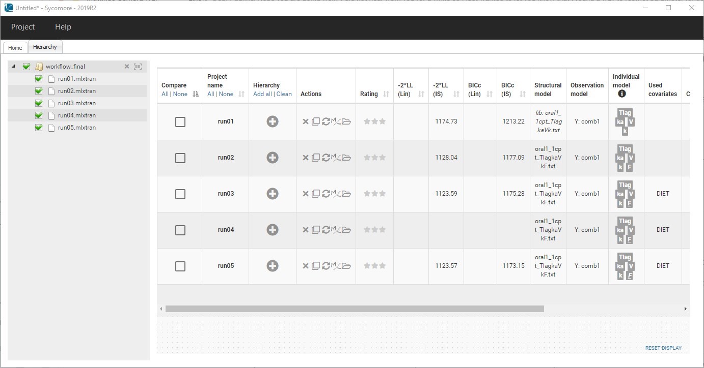
Moreover, the -2*LL and BICc for run03.mlxtran are slightly smaller than run02.mlxtran (2 points of difference), showing that the modified model still captures the data as well as the previous run. This can be seen easily by comparing the runs in Sycomore:
Estimation without simulated annealing
Finally, in the next step we are going to check more precisely whether some random effects are not well estimated and should be removed.
For the next run, we are going to modify the settings of SAEM to disable the simulated annealing:
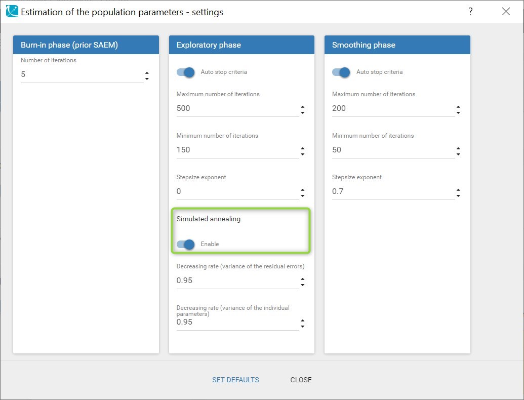
This option is explained in details in this video. Briefly, it constrains the variance of the random effects to decrease slowly during the estimation, in order to explore a large parameter space to avoid getting stuck in a local maximum. A side-effect of the simulated annealing is that it may keep the omega values artificially high, and prevent the identification of parameters for which the variability is in fact zero. This leads to large values in the standard errors. So when large standard errors are estimated for random effects, like it is the case here for omega_ka and gamma_F, it is recommended to disable the simulated annealing once the estimated parameters are close to the solution.
Before changing the settings, the last estimates should be used as new initial values to start really close to the solution. The modified project is saved as run04.mlxtran and SAEM is run. In the graphical report, omega_ka and gamma_F now decrease to a very small value:
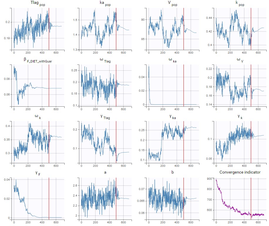
This confirms that there is not enough information in the data to identify the distributions for ka and F. Therefore, we can use the last estimates and then remove the IIV on ka and the IOV on F. The IOV on F can be removed while keeping the covariate effect of DIET, because F has also no IIV.
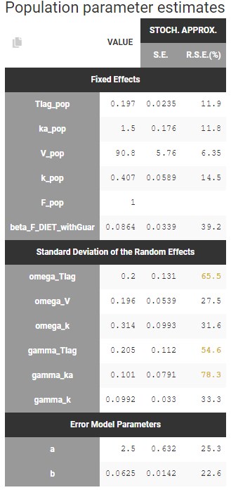
After doing this, we run the whole scenario again for the new project run05.mlxtran. All the parameters are now estimated with quite good standard errors, considering the small size of the data:
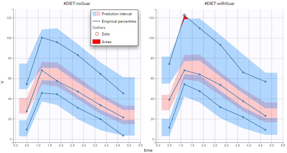
With the covariate effect on DIET on F, the discrepancy in the VPC for the occasions with guar gum is slightly smaller but still present, and is likely due to the variability in the data:
This run is the final model. Despite the small size of the data, it is able to take into account IIV and IOV, and to explain a modest part of the inter-occasion variability in bioavailability of alcohol by the effect of guar gum.