PK model: single route of administration using Monolix

Introduction
- the pkmodel function
Intravenous bolus injection
Intravenous infusion
Oral administration
Using different parametrizations

Objectives: learn how to define and use a PK model for single route of administration.

Projects: bolusLinear_project, bolusMM_project, bolusMixed_project, infusion_project, oral1_project, oral0_project, sequentialOral0Oral1_project, simultaneousOral0Oral1_project, oralAlpha_project, oralTransitComp_project

Introduction

Once a drug is administered, we usually describe subsequent processes within the organism by the pharmacokinetics (PK) process known as ADME: absorption, distribution, metabolism, excretion. A PK model is a dynamical system mathematically represented by a system of ordinary differential equations (ODEs) which describes transfers between compartments and elimination from the central compartment.
Mlxtran is remarkably efficient for implementing simple and complex PK models:

The function pkmodel can be used for standard PK models. The model is defined according to the provided set of named arguments. The pkmodel function enables different parametrizations, different models of absorption, distribution and elimination, defined here and summarized in the following..
PK macros define the different components of a compartmental model. Combining such PK components provide a high degree of flexibility for complex PK models. They can also extend a custom ODE system.
A system of ordinary differential equations (ODEs) can be implemented very easily.

It is also important to highlight the fact that the data file used by Monolix for PK modelling only contains information about dosing, i.e. how and when the drug is administrated. There is no need to integrate in the data file any information related to the PK model. This is an important remark since it means that any (complex) PK model can be used with the same data file. In particular, we make a clear distinction between administration (related to the data) and absorption (related to the model).

The pkmodel function

The PK model is defined by the names of the input parameters of the pkmodel function. These names are reserved keywords.

Absorption

p: Fraction of dose which is absorbed
ka: absorption constant rate (first order absorption)
or, Tk0: absorption duration (zero order absorption)
Tlag: lag time before absorption
or, Mtt, Ktr: mean transit time & transit rate constant

Distribution

V: Volume of distribution of the central compartment
k12, k21: Transfer rate constants between compartments 1 (central) & 2 (peripheral)
or V2, Q2: Volume of compartment 2 (peripheral) & inter compartment clearance, between compartments 1 and 2,
k13, k31: Transfer rate constants between compartments 1 (central) & 3 (peripheral)
or V3, Q3: Volume of compartment 3 (peripheral) & inter compartment clearance, between compartments 1 and 3.

Elimination

k: Elimination rate constant
or Cl: Clearance
Vm, Km: Michaelis Menten elimination parameters

Effect compartment

ke0: Effect compartment transfer rate constant

Intravenous bolus injection

Linear elimination

bolusLinear_project

A single iv bolus is administered at time 0 to each patient. The data file bolus1_data.txt contains 4 columns: id, time, amt (the amount of drug in mg) and y (the measured concentration). The names of these columns are recognized as keywords by Monolix:
It is important to note that, in this data file, a row contains either some information about the dose (in which case y = ".") or a measurement (in which case amt = "."). We could equivalently use the data file bolus2_data.txt which contains 2 additional columns: EVID (in the green frame) and IGNORED OBSERVATION (in the blue frame):

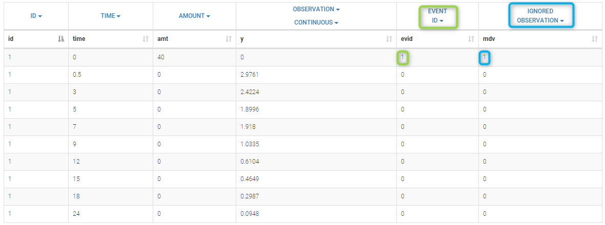Here, the EVENT ID column allows the identification of an event. It is an integer between 0 and 4. It helps to define the type of line. EVID=1 means that this record describes a dose while EVID=0 means that this record contains an observed value.
On the other hand, the IGNORED OBSERVATION column enables to tag lines for which the information in the OBSERVATION column-type is missing. MDV=1 means that the observed value of this record should be ignored while MDV=0 means that this record contains an observed value. The two data files bolus1_data.txt and bolus2_data.txt contain exactly the same information and provide exactly the same results. A one compartment model with linear elimination is used with this project:

$$\begin{array}{ccl} \frac{dA_c}{dt} &=& – k A_c(t) \\ A_c(t) &= &0 ~~\text{for}~~ t<0 \end{array} $$

Here, $A_c(t)$ and $C_c(t)=A_c(t)/V$ are, respectively, the amount and the concentration of drug in the central compartment at time t. When a dose D arrives in the central compartment at time $\tau$, an iv bolus administration assumes that

$$A_c(\tau^+) = A_c(\tau^-) + D$$

where $A_c(\tau^-)$ (resp. $A_c(\tau^+)$) is the amount of drug in the central compartment just before (resp. after) $\tau$ Parameters of this model are V and k. We therefore use the model bolus_1cpt_Vk from the Monolix PK library:

[LONGITUDINAL]
input = {V, k}

EQUATION:
Cc = pkmodel(V, k)

OUTPUT:
output = Cc

We could equivalently use the model bolusLinearMacro.txt (click on the button Model and select the new PK model in the library 6.PK_models/model)

[LONGITUDINAL]
input = {V, k}

PK:
compartment(cmt=1, amount=Ac)
iv(cmt=1)
elimination(cmt=1, k)
Cc = Ac/V

OUTPUT:
output = Cc

These two implementations generate exactly the same C++ code and then provide exactly the same results. Here, the ODE system is linear and Monolix uses its analytical solution. Of course, it is also possible (but not recommended with this model) to use the ODE based PK model bolusLinearODE.txt :

[LONGITUDINAL]
input = {V, k}

PK:
depot(target = Ac)

EQUATION:
ddt_Ac = - k*Ac
Cc = Ac/V

OUTPUT:
output = Cc

Results obtained with this model are slightly different from the ones obtained with the previous implementations since a numeric scheme is used here for solving the ODE. Moreover, the computation time is longer (between 3 and 4 time longer in that case) when using the ODE compared to the analytical solution.
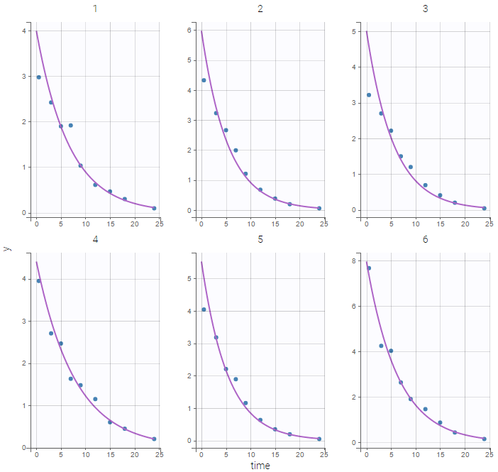
Individual fits obtained with this model look nice

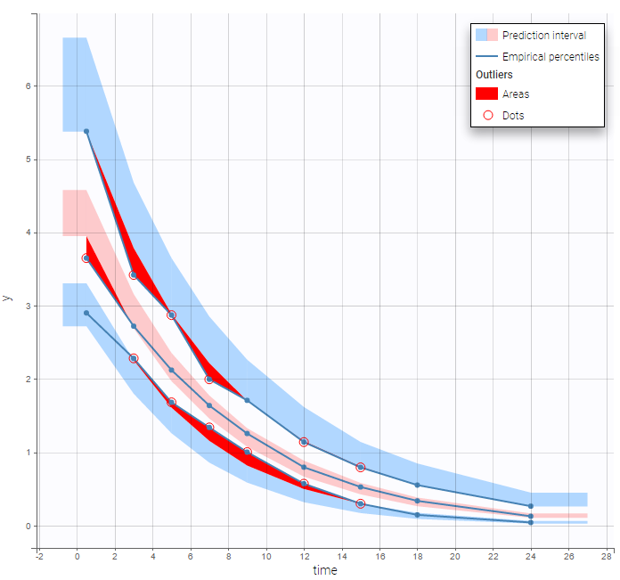
but the VPC show some misspecification in the elimination process:

Michaelis Menten elimination

bolusMM_project

A non linear elimination is used with this project:

$$\frac{dA_c}{dt} = – \frac{ V_m \, A_c(t)}{V\, K_m + A_c(t) }$$

This model is available in the Monolix PK library as bolus_1cpt_VVmKm:

[LONGITUDINAL]
input = {V, Vm, Km}

PK:
Cc = pkmodel(V, Vm, Km)

OUTPUT:
output = Cc

Instead of this model, we could equivalently use PK macros with bolusNonLinearMacro.txt from the library 6.PK_models/model:

[LONGITUDINAL]
input = {V, Vm, Km}

PK:
compartment(cmt=1, amount=Ac, volume=V)
iv(cmt=1)
elimination(cmt=1, Vm, Km)
Cc = Ac/V

OUTPUT:
output = Cc

or an ODE with bolusNonLinearODE:

[LONGITUDINAL]
input = {V, Vm, Km}

PK:
depot(target = Ac)

EQUATION:
ddt_Ac = -Vm*Ac/(V*Km+Ac) 
Cc=Ac/V

OUTPUT:
output = Cc

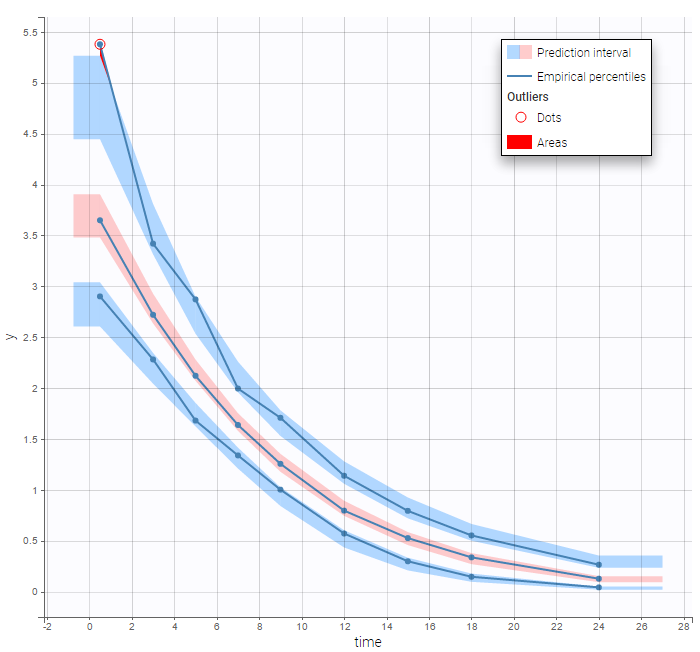
Results obtained with these three implementations are identical since no analytical solution is available for this non linear ODE. We can then check that this PK model seems to describe much better the elimination process of the data:

Mixed elimination

bolusMixed_project

THe Monolix PK library contains “standard” PK models. More complex models should be implemented by the user in a model file. For instance, we assume in this project that the elimination process is a combination of linear and nonlinear elimination processes:

$$ \frac{dA_c}{dt} = -\frac{ V_m A_c(t)}{V K_m + A_c(t) } – k A_c(t) $$

This model is not available in the Monolix PK library. It is implemented in bolusMixed.txt:

[LONGITUDINAL]
input = {V, k, Vm, Km}

PK:
depot(target = Ac)

EQUATION:
ddt_Ac = -Vm*Ac/(V*Km+Ac) - k*Ac
Cc=Ac/V

OUTPUT:
output = Cc

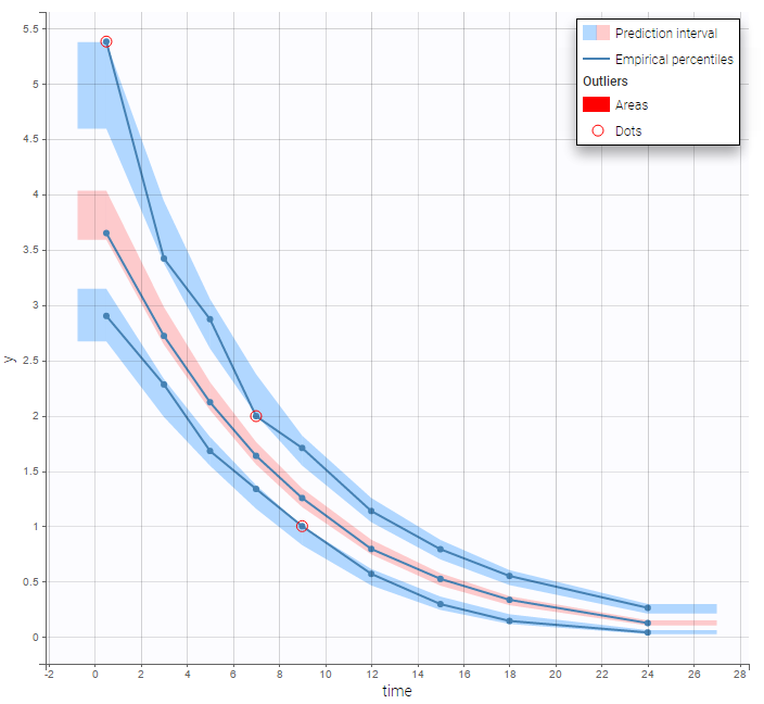
This model, with a combined error model, seems to describe very well the data:

Intravenous infusion

infusion_project

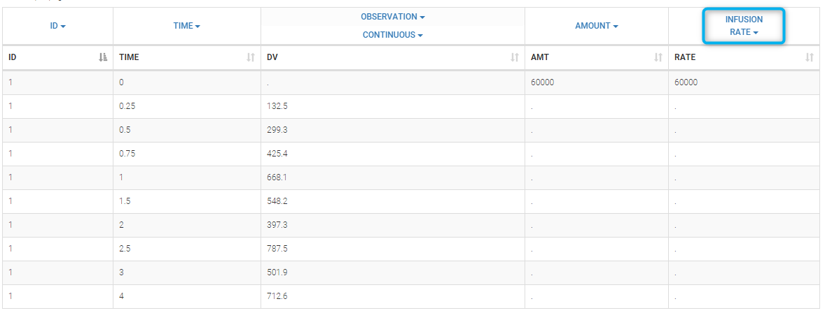
Intravenous infusion assumes that the drug is administrated intravenously with a constant rate (infusion rate), during a given time (infusion time). Since the amount is the product of infusion rate and infusion time, an additional column INFUSION RATE or INFUSION DURATION is required in the data file: Monolix can use both indifferently. Data file infusion_rate_data.txt has an additional column rate:

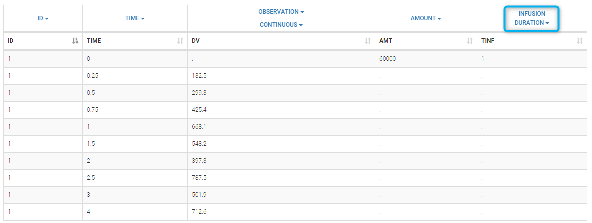
It can be replaced by infusion_tinf_data.txt which contains exactly the same information:

We use with this project a 2 compartment model with non linear elimination and parameters $V_1$ , $Q$ , $V_2$ , $V_m$ , $K_m$ :

$$\begin{aligned} k_{12} &= Q/V_1 \\ k_{21} &= Q/V_2 \\\frac{dA_c}{dt} & = k_{21} \, Ap(t) – k_{12} \, Ac(t)- \frac{ V_m \, A_c(t)}{V_1\, K_m + A_c(t) } \\ \frac{dA_p}{dt} & = – k_{21} \, Ap(t) + k_{12} \, Ac(t) \\ Cc(t) &= \frac{Ac(t)}{V_1} \end{aligned}$$

This model is available in the Monolix PK library as infusion_2cpt_V1QV2VmKm:

[LONGITUDINAL]
input = {V1, Q, V2, Vm, Km}

PK:
V = V1
k12 = Q/V1
k21 = Q/V2
Cc = pkmodel(V, k12, k21, Vm, Km)

OUTPUT:
output = Cc

Oral administration

first-order absorption

oral1_project

This project uses the data file oral_data.txt. For each patient, information about dosing is the time of administration and the amount. A one compartment model with first order absorption and linear elimination is used with this project. Parameters of the model are ka, V and Cl. we will then use model oral1_kaVCl.txt from the Monolix PK library

[LONGITUDINAL]
input = {ka, V, Cl}

EQUATION:
Cc = pkmodel(ka, V, Cl)

OUTPUT:
output = Cc

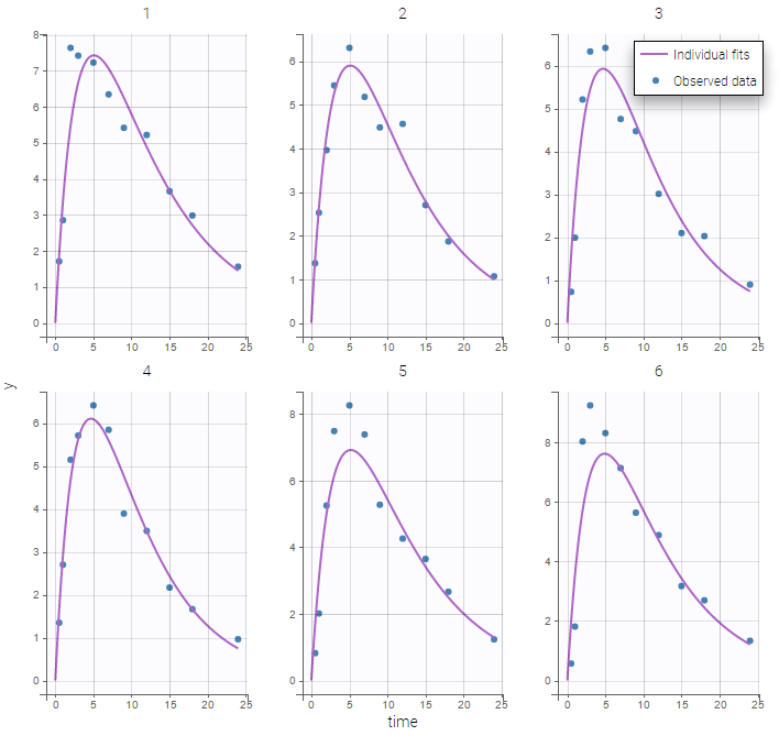
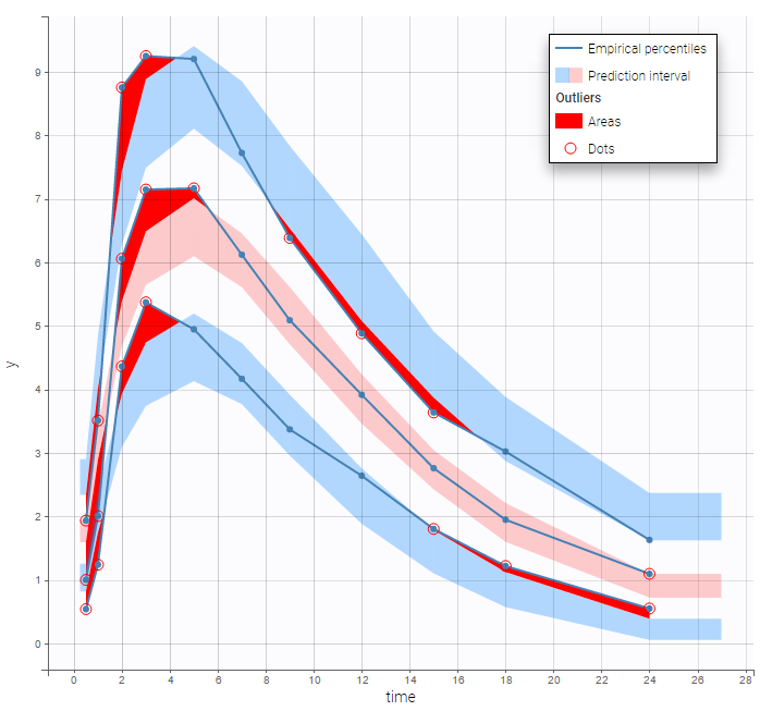
Both the individual fits and the VPCs show that this model doesn’t describe the absorption process properly.

Many options for implementing this PK model with Mlxtran exists:
– using PK macros: oralMacro.txt:

[LONGITUDINAL]
input = {ka, V, Cl}

PK:
compartment(cmt=1, amount=Ac)
oral(cmt=1, ka)
elimination(cmt=1, k=Cl/V) 
Cc=Ac/V

OUTPUT:
output = Cc

– using a system of two ODEs as in oralODEb.txt:

[LONGITUDINAL]
input = {ka, V, Cl}

PK:
depot(target=Ad)

EQUATION:
k = Cl/V
ddt_Ad = -ka*Ad
ddt_Ac =  ka*Ad - k*Ac
Cc = Ac/V

OUTPUT: 
output = Cc

– combining PK macros and ODE as in oralMacroODE.txt (macros are used for the absorption and ODE for the elimination):

[LONGITUDINAL]
input = {ka, V, Cl}

PK:
compartment(cmt=1, amount=Ac)
oral(cmt=1, ka)

EQUATION:
k = Cl/V
ddt_Ac = - k*Ac
Cc = Ac/V

OUTPUT: 
output = Cc

– or equivalently, as in oralODEa.txt:

[LONGITUDINAL]
input = {ka, V, Cl}

PK:
depot(target=Ac, ka)

EQUATION:
k = Cl/V
ddt_Ac = - k*Ac
Cc = Ac/V<

OUTPUT: 
output = Cc

Remark: Models using the pkmodel function or PK macros only use an analytical solution of the ODE system.

zero-order absorption

oral0_project

A one compartment model with zero order absorption and linear elimination is used to fit the same PK data with this project. Parameters of the model are Tk0, V and Cl. We will then use model oral0_1cpt_Tk0Vk.txt from the Monolix PK library

[LONGITUDINAL]
input = {Tk0, V, Cl}

EQUATION:
Cc = pkmodel(Tk0, V, Cl)

OUTPUT:
output = Cc

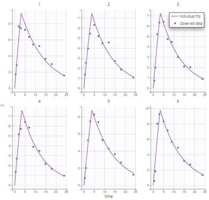
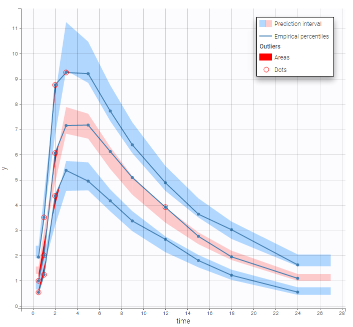
Remark 1: implementing a zero-order absorption process using ODEs is not easy… on the other hand, it becomes extremely easy to implement using either the pkmodel function or the PK macro oral(Tk0).
Remark 2: The duration of a zero-order absorption has nothing to do with an infusion time: it is a parameter of the PK model (exactly as the absorption rate constant ka for instance), it is not part of the data.

sequential zero-order first-order absorption

sequentialOral0Oral1_project

More complex PK models can be implemented using Mlxtran. A sequential zero-order first-order absorption process assumes that a fraction Fr of the dose is first absorbed during a time Tk0 with a zero-order process, then, the remaining fraction is absorbed with a first-order process. This model is implemented in sequentialOral0Oral1.txt using PK macros:

[LONGITUDINAL]
input = {Fr, Tk0, ka, V, Cl}

PK:
compartment(amount=Ac)
absorption(Tk0, p=Fr)
absorption(ka, Tlag=Tk0, p=1-Fr)
elimination(k=Cl/V)
Cc=Ac/V

OUTPUT:
output = Cc

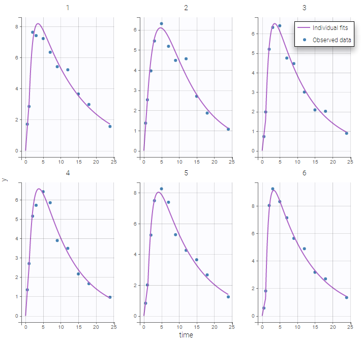
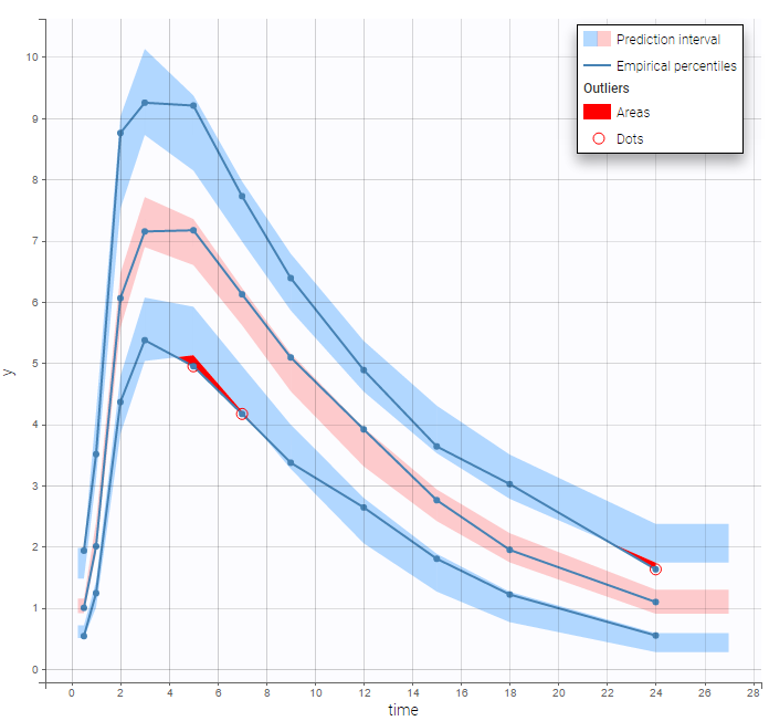
Both the individual fits and the VPCs show that this PK model describes very well the whole ADME process for the same PK data:

simultaneous zero-order first-order absorption

simultaneousOral0Oral1_project

A simultaneous zero-order first-order absorption process assumes that a fraction Fr of the dose is absorbed with a zero-order process while the remaining fraction is absorbed simultaneously with a first-order process. This model is implemented in simultaneousOral0Oral1.txt using PK macros:

[LONGITUDINAL]
input = {Fr, Tk0, ka, V, Cl}

PK:
compartment(amount=Ac)
absorption(Tk0, p=Fr)
absorption(ka, p=1-Fr)
elimination(k=Cl/V)
Cc=Ac/V

OUTPUT:
output = Cc

alpha-order absorption

oralAlpha_project

An $\alpha$ -order absorption process assumes that the rate of absorption is proportional to some power of the amount of drug in the depot compartment:

$\frac{dA_d}{dt} = - r \left(A_d(t)\right)^\alpha$

This model is implemented in oralAlpha.txt using ODEs:

[LONGITUDINAL]
input = {r, alpha, V, Cl}

PK:
depot(target = Ad)

EQUATION:
dAd = Ad^alpha
ddt_Ad = -r*dAd
ddt_Ac = r*Ad - (Cl/V)*Ac
Cc = Ac/V

OUTPUT:
output = Cc

transit compartment model

oralTransitComp_project

A PK model with a transit compartment of transit rate Ktr and mean transit time Mtt can be implemented using the PK macro oral(ka, Mtt, Ktr), or using the pkmodel function, as in oralTransitComp.txt:

[LONGITUDINAL]
input = {Mtt, Ktr, ka, V, Cl}

EQUATION:
Cc = pkmodel(Mtt, Ktr, ka, V, Cl)

OUTPUT:
output = Cc

Using different parametrizations

The PK macros and the function pkmodel use some preferred parametrizations and some reserved names as input arguments: Tlag, ka, Tk0, V, Cl, k12, k21. It is however possible to use another parametrization and/or other parameter names. As an example, consider a 2-compartment model for oral administration with a lag, a first order absorption and a linear elimination. We can use the pkmodel function with, for instance, parameters ka, V, k, k12 and k21:

[LONGITUDINAL]
input = {ka, V, k, k12, k21}

PK:
Cc = pkmodel(ka, V, k, k12, k21)

OUTPUT:
output = Cc

Imagine now that we want i) to use the clearance $Cl$ instead of the elimination rate constant $k$ , ii) to use capital letters for the parameter names. We can still use the pkmodel function as follows:

[LONGITUDINAL]
input = {KA, V, CL, K12, K21}

PK:
Cc = pkmodel(ka=KA, V, k=CL/V, k12=K12, k21=K21)

OUTPUT:
output = Cc