How to compute additional outputs such as AUC and Cmax in the structural model

Computing additional outputs such as AUC and Cmax in the structural model is possible but requires a particular syntax, because it is not possible to redefine a variable in Mlxtran. For example, it would not be possible to directly update the variable Cmax = Cc when Cc>Cmax. But it is possible to compute Cmax via an ODE, where Cmax increases like Cc at each time where Cc>Cmax. This page gives detailed examples for the AUC on full time interval or specific interval, Cmax, nadir, and other derived variables such as duration above a threshold.

AUClast on full time interval
Time interval AUC
Dose interval AUC (AUCtau)
Cmax or nadir
Time above a threshold
Time since disease progression

Often the Area under the PK curve (AUC) is needed as an important PK metric to link with the pharmacodynamic effect. We show here how to:

compute the AUC within the mlxtran model file
output the AUC calculations for later analysis.

Calculation of the AUC can be done in the EQUATION section of the Mlxtran model. If a dataset contains the AUC observations, then the calculation in the EQUATION section can be used as an output in the output={} definition (matched to observations of the data set). Or it can be saved for post-treatment using table={}, as described here.

AUClast from t=0 to t=tlast

The following code is the basic implementation of the AUC for a 1-compartmental model with the absorption rate ka. It integrates the concentration profile from the start to the end of the observation period.

[LONGITUDINAL]
input = {ka, V, Cl}

PK:
Cc=pkmodel(ka,V,Cl)

EQUATION:
odeType=stiff
ddt_AUC = Cc

OUTPUT:
output = {Cc}
table  = {AUC}

AUC in a time interval

The following code computes the AUC between two time points t1 and t2. The idea is to compute the AUC_0_t1 and AUC_0_t2 using if/else statements and then do the difference between the two.

[LONGITUDINAL]
input = {ka, V, Cl}
PK:
depot(ka, target=Ac)

EQUATION:
odeType = stiff
useAnalyticalSolution=no

Cc = pkmodel(ka,V,Cl)

t1=24
t2=48
AUCt1_0 = 0
if(t < t1)
   dAUCt1 = Cc
else
   dAUCt1 = 0
end
ddt_AUCt1 = dAUCt1

AUCt2_0 = 0
if(t < t2)
   dAUCt2 = Cc
else
   dAUCt2 = 0
end
ddt_AUCt2 = dAUCt2

AUC_t1_t2 = AUCt2 - AUCt1

OUTPUT:
output = {Cc}
table  = {AUC_t1_t2}

Note that the t==tDose would not work because the integrator does not necessarily evaluate the time exactly at the times of doses. Thus the test t==tDose might not be tested at all during the computation.
Also note that, although partial AUC can be calculated by comparing time with the both boundaries in the if statement (e.g. if (t>20 and t<40)), this might not be the best practice when concentration is calculated using an analytical solution, because ODE solver used for calculating AUC could be deceived by AUC remaining 0 for a period of time and might increase the integration time step to a value larger than the difference between time boundaries.

Dose-interval AUC (AUCtau)

The following code compute the AUCtau for each dose interval. At each dose the AUC is reset to zero and the concentration is integrated until the next administration.

[LONGITUDINAL]
input = {ka, V, Cl}

PK:
Cc = pkmodel(ka,V,Cl)

; Reset the ODE variable AUCtau to zero each time there is a dose
empty(target=AUCtau)

EQUATION: 
odeType=stiff
ddt_AUCtau = Cc 

OUTPUT: 
output = {Cc} 
table = {AUCtau}

Since AUCtau is equal to 0 at each dosing time as it has just been reset, the AUC in the last interdose interval should actually be read just before that time.

Here we provide a Simulx project with an example of a PK model where AUCtau is calculated as additional lines in the model and defined as an output of the simulations.

Computing the Cmax or nadir in the structural model

Cmax

Cmax can be calculated directly in the structural model by integrating the increase of the concentration. Alternatively, the Cmax can also be calculated in Simulx using the Outcomes&Endpoints tab.

Cmax for models with first-order absorption

The following example shows how to do it in case of a one-compartment model with first-order absorption and linear elimination. Absorption processes defined via the depot macro must be replaced by explciit ODEs, while the depot macro is used to add the dose as a bolus into the depot compartment.

[LONGITUDINAL]
input = {Cl, ka, V}

PK:
depot(target=Ad)

EQUATION:

; initial conditions
t_0  = 0
Ad_0 = 0
Ac_0 = 0

ddt_Ad = -ka*Ad
ddt_Ac = ka*Ad - k*Ac
Cc = Ac/V

; Calculation of Cmax
slope  = ka*Ad -k*Ac
Cmax_0 = 0
if slope > 0 && Cc > Cmax
   x = slope/V
else
   x = 0
end

ddt_Cmax = x

Cmax for model with bolus administration or infusion

If the dose is administered as bolus, it is necessary to add in the model a very short infusion. This prevents from the instantaneous increase of the concentration. The following example shows this situations in case of a three-compartments model with linear elimination. The duration of the “short infusion” can be adapted with respect to the time scale by modifying dT=0.1.

If the doses are administered via iv infusion, then dT=0.1 can be replaced by dT = inftDose, which reads the infusion duration from the data.

[LONGITUDINAL]
input = {Cl, V1, Q2, V2, Q3, V3}

EQUATION:

; Parameter transformations 
V   = V1 
k   = Cl/V1 
k12 = Q2/V1 
k21 = Q2/V2 
k13 = Q3/V1 
k31 = Q3/V3

; initial conditions
t_0  = 0
Ac_0 = 0
A2_0 = 0
A3_0 = 0

;short pseudo-infusion duration
dT = 0.1 ; use dT=inftDose if the administration is infusion: inftDose is the infusion duration from the last dose read from the data

; infusion input to Ac
if t < tDose+dT
   input = amtDose/dT ;amtDose is the last dose amount read from the data
else
   input = 0
end

dAc = input -k*Ac - k12*Ac - k13*Ac + k21*A2 + k31*A3
ddt_Ac = dAc
ddt_A2 = k12*Ac - k21*A2
ddt_A3 = k13*Ac - k31*A3
Cc = Ac/V

; Calculation of AUC
AUC_0 = 0
ddt_AUC = Cc

; Calculation of Cmax
Cmax_0 = 0
if dAc > 0 && Cc > Cmax
   x = dAc/V
else
   x = 0
end

ddt_Cmax = x

OUTPUT:
output = {Ac, Cc}
table  = {Cmax, AUC}

Cmax for models with transit compartments

The transit compartments defined via the depot() macro must be replaced by explicit ODEs. The amount in the last (nth) transit compartment is described via an analytical solution using the keyword amtDose to get the dose amount and (t-tDose) to get the time elapsed since the last dose. The calculation of Cmax then follows the same logic as for a first-order absorption.

[LONGITUDINAL]
input={F, Ktr, Mtt, ka, V, Cl}

EQUATION:
k = Cl/V
odeType=stiff

; transit model with explicit ODEs
n = max(0, Mtt*Ktr - 1)
An = F * amtDose * exp( n * log(Ktr*(t-tDose)) - factln(n) - Ktr * (t-tDose))

t_0 = 0
Aa_0 = 0
Ac_0 = 0

ddt_Aa = Ktr*An - ka*Aa
ddt_Ac = ka*Aa - k*Ac
Cc = Ac/V

; Calculation of Cmax
slope  = ka*Aa - k*Ac
Cmax_0 = 0
if slope > 0 && Cc > Cmax
   x = slope/V
else
   x = 0
end

ddt_Cmax = x

OUTPUT:
output = {Cc}
table = {Cmax}

Nadir

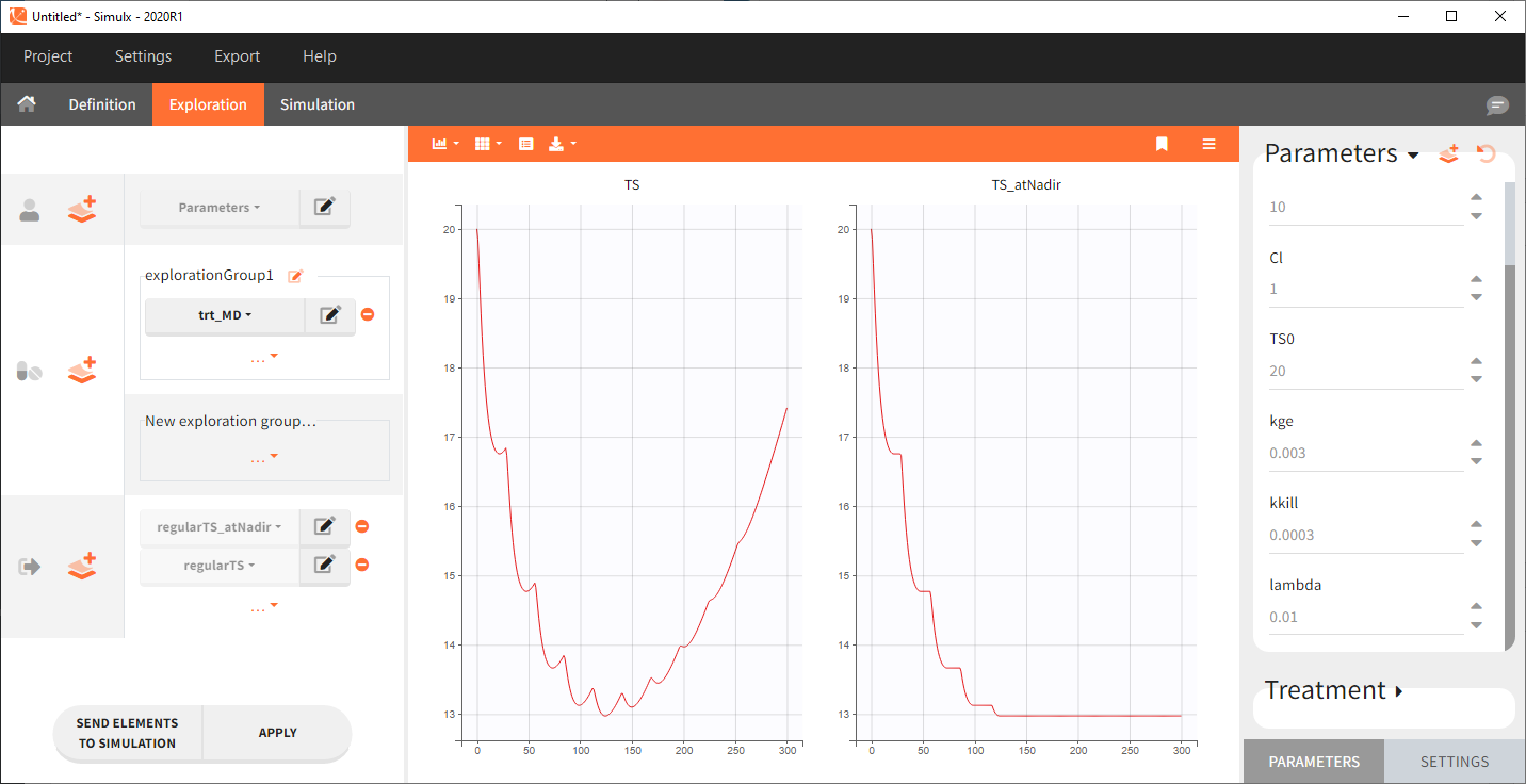
This example shows how to compute tumor size (variable TS) at time of nadir:

[LONGITUDINAL]
input = {ka, Vl, Cl, TS0, kge, kkill, lambda}
EQUATION:

odeType=stiff
Cc = pkmodel(ka, V, Cl)

; ODE system for tumor growth dynamics
t_0 = 0
TS_0 = TS0
TSDynamics = (kge*TS)-kkill*TS*Cc*exp(-lambda*t)
ddt_TS = TSDynamics

; ===== computing TS at nadir
if TSDynamics < 0 && TS < TS_atNadir
  x = TSDynamics
else
  x = 0
end
TS_atNadir_0 = TS0
ddt_TS_atNadir = x

OUTPUT:
output = {TS}
table = {TS_atNadir}

Here is an example of simulation for TS and TS_atNadir with a multiple dose schedule:

Time above a threshold

Here we compute the time that a variable C spends above some threshold, which could be a toxicity threshold for example. This piece of code comes in the structural model, after the dynamics of the variable C has already been defined.

TimeAboveThreshold_0 = 0
if C > Cthreshold
  xTime = 1
else
  xTime = 0
end
ddt_TimeAboveThreshold = xTime

Time since disease progression

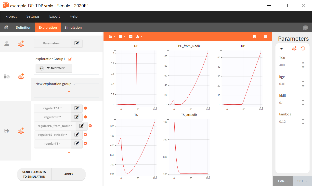
In this full structural model example, tumor size TS is described with an exponential growth, and a constant treatment effect since time=0 with a log-kill killing hypothesis and a Claret exponential resistance term. Several additional variables are computed:

TS_atNadir: the tumor size at the time of nadir,
PC_from_Nadir: the percent change of TS between the time of nadir and the current time,
DP: predicted disease progression status (1 if TS has increased more than >20% and >5-mm from last nadir, 0 otherwise),
TDP: time since disease progression (duration since last time when DP is switched from 0 to 1)

[LONGITUDINAL]
input = {TS0, kge, kkill, lambda}

EQUATION:
odeType=stiff

;initial conditions:
;t_0 = 0 ;this should be uncommented if the initial time is 0 for all subjects 
TS_0 = TS0

K = kkill*exp(-lambda*t)

;Saturation for TS at 1e12 to avoid infinite values
if TS>1e12
  TSDynamics = 0
  else
  if t<0 ; before treatment
    TSDynamics = (kge*TS)
  else ; after treatment
    TSDynamics = (kge*TS)-K*TS
  end
end

ddt_TS = TSDynamics

; Computing time to nadir (TS decreases after treatment start at time=0, then increases again because of resistance)
if TSDynamics<0
  x1=1
else
  x1=0
end
TimeToNadir_0=t0
ddt_TimeToNadir = x1 ; x1 is used as intermediate variable because it is not possible to define an ODE inside an if/else statement

; Computing TS at time of nadir
if TSDynamics < 0 & TS < TS_atNadir
  x2 = TSDynamics
else
  x2 = 0
end
TS_atNadir_0 = TS0
ddt_TS_atNadir = x2 ;

; Computing DP: predicted disease progression status at the previous visit (1 if TS has increased more than >20% and >5-mm from last nadir, 0 otherwise)
PC_from_Nadir = (TS/TS_atNadir-1)*100
if t>TimeToNadir & PC_from_Nadir > 20 & (TS-TS_atNadir) > 5
  DP = 1
else
  DP = 0
end

; Computing TDP = time since disease progression: duration since last time DP was switched from 0 to 1
if DP==1
  x3 = 1
else
  x3 = 0
end
TDP_0 = 0
ddt_TDP = x3

OUTPUT: 
output = {TS}
table = {TS_atNadir, PC_from_Nadir, DP, TDP}

Simulx can be conveniently used to simulate each intermediate variable with typical parameters (the example model and Simulx project can be downloaded here):