Individual fits

Purpose

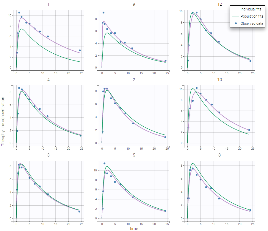
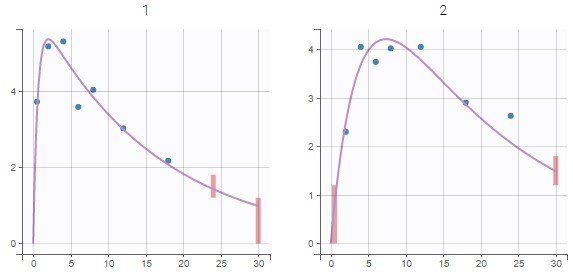
The figure displays the observed data for each subject, as well as two curves from simulations using the design and the covariates of each subject:

• the predicted profile given by the estimated population model (Population fits),
• the predicted profile given by the estimated individual model (Individual fits). If the EBEs and/or the conditional distribution tasks were performed, the user can choose either the conditional means or the conditional modes, estimated by MCMC, as estimators. Otherwise, approximations of the conditional means from SAEM are used.

This is a good way to see on each subject the validity of the model, and the actual fit proposed, as well as the inter-individual variability in the kinetics. It is possible to show the computed individual parameters on the figure. Moreover, it is also possible to display an individual predictive check: the median and a confidence interval for () estimated with a Monte Carlo procedure.

Examples

• Individual fits and population fits

In the example below, the concentration for the theophylline data set is shown with simulations of a one-compartment model with first-order absorption and linear elimination. For each subject, the data are displayed with blue points along with the individual fit and population fit (the prediction using the estimated individual and population parameters respectively).

• Individual parameters

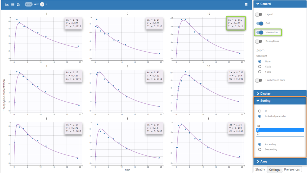
Information on individual parameters can be used in two ways, as shown below. By clicking on Information (marked in green on the figure) in the General panel, individual parameter values can be displayed on each individual plot. Moreover, the plots can be sorted according to the values for a given parameter, in ascending or descending order (Sorting panel marked in orange). By default, the individual plots are sorted by subject id, with the same order as in the data set.

• Individual predictive check

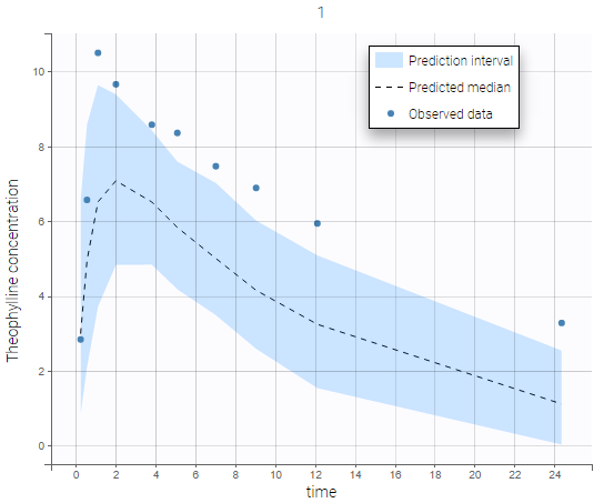
Individual predictive checks can be added to the plots: for each individual a prediction interval is computed based on multiple simulations with the population parameters and the design structure of this individual. The median line of the interval is also drawn. The interval allows to check whether the observed data are compatible with the population prediction, taking into account the inter-individual variability. The example below shows that the first subject in the theophylline data set show too much variability from the rest of the population to be correctly described by the population model.

• Dosing times

Dosing times can also be overlayed, which is useful to visualize the effect of doses on the prediction. As an example, the following figure shows the observations of an individual from the tobramycin data set along with the corresponding individual fit and multiple dosing times. Starting in version 2021R1 on, dosing times corresponding to doses with null amounts are not displayed.

• Special zoom

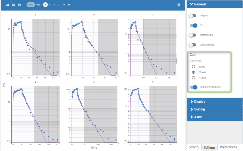
User-defined constraints for the zoom are available. They allow to zoom in according to one axis only instead of both axes. Moreover, a link between plots can be set in order to perform a linked zoom on all individual plots at once. This is shown on the figure below with observations from the remifentanil example, and individual fits from a two-compartment model. It is thus possible to focus on the same time range or observation values for all individuals. In this example it is used to zoom on time on the elimination phase for all individuals, while keeping the Y axis in log scale unchanged for each plot.

• Censored data

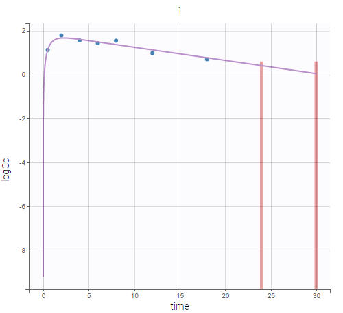
When a data is censored, this data is different to a “classical” observation and has thus a different representation. We represent it as a bar from the censored value specified in the data set and the associated limit.

If there is no limit column then is goes to Infinity as in the following example. However, in any case, the user can choose the limit of the plot.

Settings

• Grid arrange. The user can define the number of subjects that are displayed, as well as the number of rows and the number of columns. Moreover, a slider is present to be able to change the subjects under consideration.
• General
  • Legend: hide/show the legend. The legends adapts automatically to the elements displayed on the plot. The same legend box applies to all subplots and it is possible to drag and drop the legend at the desired place.
  • Grid : hide/show the grid in the background of the plots.
  • Information: hide/show the individual parameter values for each subject (conditional mode or conditional mean depending on the “Individual estimates” choice is the setting section “Display”).
  • Dosing times: hide/show dosing times as vertical lines for each subject.
  • Link between plots: activate the linked zoom for all subplots. The same zooming region can be applied on all individuals only on the x-axis, only on the Y-axis or on both (option “none”).
• Display
  • Observed data: hide/show the observed data.
  • Censored intervals [if censored data present]: hide/show the data marked as censored (BLQ), shown as a rectangle representing the censoring interval (for instance [0, LOQ]).
  • Split occasions [if IOV present]: Split the individual subplots by occasions in case of IOV.
  • Individual fits: Model prediction for each individual using the subject’s design and the individual parameters. The individual parameters can be the conditional mode or the conditional mean depending on the choice in the “Individual estimates” section.
  • Population fits [if no covariates in the model]: Model prediction for each individual using the subject’s design and the population parameters.
  • Population fits (individual covariates) [if covariates present in the model]: Model prediction for each individual using the subject’s design, the population parameters and the individual covariates values.
  • Population fits (population covariates) [if covariates present in the model]: Model prediction for each individual using the subject’s design, the population parameters and the median covariates values (median from all individuals of the data set).
  • Individual estimates [if EBEs task has run]: depending on the tasks that have been calculated, choice between conditional mode (given by EBEs task), conditional mean (approximation given by the population parameter estimated task) or conditional mean (given by the conditional distribution task).
  • Individual predictive check: For each individual, 500 (see “number of simulations” in the PLOTS task settings) data sets are simulated using the individual’s design (dose and regressor values). The parameter values used for the simulation include the population parameter values, the individual covariate values and random effects sampled from the population distribution. The simulated data sets include residual errors. The prediction interval represents the interval containing 90% (see “level” setting) of the simulated data points. The predicted median is the median of all simulated data points. The individual predictive check allows to visualize the inter-individual variability (unexplained by covariates) and compare the population prediction to the individual observations.
• Sorting: Sort the subjects by ID or individual parameter values in ascending or descending order.

By default, only the observed data and the individual fits are displayed.