Purpose
This plot displays the distribution of the standardized random effects with boxplots or with histograms. Since random effects should follow normal probability laws, it is useful to compare the distributions to standard Gaussian distributions.
Example
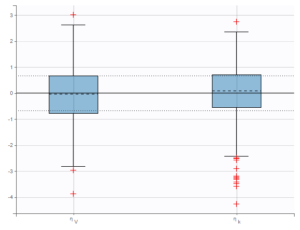
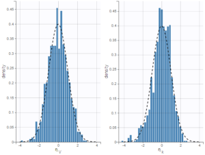
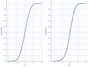
In the following example, one can see the distributions of two parameters of a two-compartment bolus model with linear elimination, estimated on the tobramycin example. On the left, the distributions are represented as boxplots, in the middle as histograms for the probability density function (PDF), and on the right as cumulative distribution functions (CDF). In each case, marks to compare the results to standard Gaussian distributions are overlaid: dotted horizontal lines indicate the interquartile interval of a standard Gaussian distribution for the boxplots, and black curves represent the PDF and CDF of a standard Gaussian distribution.
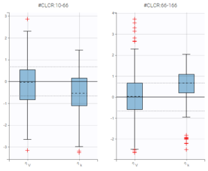
In boxplots, the dashed line represents the median, the blue box represents the 25th and 75th percentiles (Q1 and Q3), and
the whiskers extend to the most extreme data points, outliers excluded. Outliers are the points larger than Q1 + w(Q3 – Q1) or smaller than Q1 – w(Q3 – Q1) with w=1.5. Outliers are shown with red crosses.
 |
 |
 |
|---|
On the figure below, the individuals have been split into two groups according to the value of the continuous covariate CLCR. One can notice differences on the boxplots for the distributions of random effects between both groups, in particular for the parameter k.
Shrinkage
When there is not enough data to well-estimate individual parameters, individual estimates based on the conditional mean or mode (rather than the entire conditional distribution) have a tendency to shrink towards the population parameter estimate. For the distribution of the standardized random effects, shrinkage leads to bias showing less than the true variation if the individual estimates are shown using the conditional mean or conditional mode rather than the conditional distribution in this case. The shrinkage can be displayed in the plot by toggling “information” in general settings. For more details see the page Understanding shrinkage and how to circumvent it.
Settings
- General: add/remove the grid and the shrinkage in %.
- Display
- Distribution function. The user can choose which type of plot is used to represent the distributions of the random effects: boxplots, pdf (probability density function) or cdf (cumulative distribution function).
- Individual estimates. The user can define which estimator is used for the definition of the individual parameters and thus for the random effects (conditional mean, conditional mode, or conditional distribution)
- Visual cues: If boxplot has been selected, the user can choose to add or hide dotted lines to mark the median or quartiles of a standard Gaussian distribution.
By default, the distributions of simulated random effects are displayed as boxplots.
Standarized random effects in case of IOV
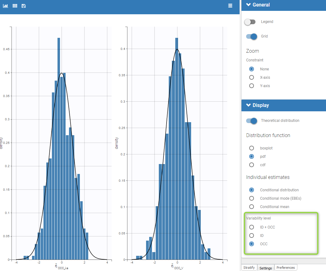
Starting from the 2019 version, in case of IOV and if the conditional distribution is computed, we propose to display the standarized random effect by level of variability. In the presented example, we put IOV on both ka and V parameters. Thus, in the plot, we proposed to display the several levels of variability for all the parameters. We can then display the standarized random effects for
- the ID level,
- the OCC level (where only the parameters with variability on this level are displayed)
- the ID+OCC level corresponding to the addition of the levels
