Probability distribution of the individual parameters in Monolix

Introduction
Marginal distributions of the individual parameters
Correlation structure of the random effects
Parameters without random effects
Custom parameter distribution

Objectives: learn how to define the probability distribution and the correlation structure of the individual parameters.

Projects: warfarin_distribution1_project, warfarin_distribution2_project, warfarin_distribution3_project, warfarin_distribution4_project

Introduction

One way to extend the use of Gaussian distributions is to consider that some transformation of the parameters in which we are interested is Gaussian, i.e., assume the existence of a monotonic function $h$ such that $h(\psi)$ is normally distributed. Then, there exists some $\omega$ such that, for each individual i:

$h(\psi_i) \sim {\cal N}(h(\bar{\psi}_i), \omega^2)$

where $\bar{\psi}_i$ is the predicted value of $\psi_i$. In this section, we consider models for the individual parameters without any covariate. Then, the predicted value of $\psi_i$ is the $\bar{\psi}_i = \psi_{\rm pop}$ and

$h(\psi_i) \sim {\cal N}(h(\psi_{pop}), \omega^2)$

The transformation $h$ defines the distribution of $\psi_i$. Some predefined distributions/transformations are available in Monolix:

Normal distribution in ]-inf,+inf[:

In that case, $h(\psi_i) = \psi_i$.
Note: the two mathematical representations for normal distributions are equivalent:

$ \psi_i \sim {\cal N}(\bar{\psi}_{i}, \omega^2) ~~\Leftrightarrow~~ \psi_i = \bar{\psi}_i + \eta_i, ~~\text{where}~~\eta_i \sim {\cal N}(0,\omega^2).$

Log-normal distribution in ]0,+inf[:

In that case, $h(\psi_i) = log(\psi_i)$. A log-normally random variable takes positive values only. A log-normal distribution looks like a normal distribution for a small variance $\omega^2$. On the other hand, the asymmetry of the distribution increases when $\omega^2$ increases.
Note: the two mathematical representations for log-normal distributions are equivalent:

$\log(\psi_i) \sim {\cal N}(\log(\bar{\psi}_{i}), \omega^2) ~~\Leftrightarrow~~ \log(\psi_i)=\log(\bar{\psi}_{i})+\eta_i~~\Leftrightarrow~~ \psi_i = \bar{\psi}_i e^{\eta_i}, ~~\text{where}~~\eta_i \sim {\cal N}(0,\omega^2).$

$\bar{\psi}_i$ represents the typical value (fixed effect) and $\omega$ the standard deviation of the random effects, which is interpreted as the inter-individual variability. Note that $\bar{\psi}_i$ is the median of the distribution (neither the mean, nor the mode).

Logit-normal distribution in ]0,1[:

In that case, $h(\psi_i) = log\left(\frac{\psi_i}{1-\psi_i}\right)$. A random variable $\psi_i$ with a logit-normal distribution takes its values in ]0,1[. The logit of $\psi_i$ is normally distributed, i.e.,

$\text{logit}(\psi_i) = \log \left(\frac{\psi_i}{1-\psi_i}\right) \ \sim \ \ {\cal N}( \text{logit}(\bar{\psi}_i), \omega^2) ~~\Leftrightarrow~~ \text{logit}(\psi_i) = \text{logit}(\bar{\psi}_i) + \eta_i, ~~\text{where}~~\eta_i \sim {\cal N}(0,\omega^2)$

Note that:

$ m = \text{logit}(\psi_i) = \log \left(\frac{\psi_i}{1-\psi_i}\right) ~~\Leftrightarrow~~ \psi_i = \frac{\exp(m)}{1+\exp(m)} $

Generalized logit-normal distribution in ]a,b[:

In that case, $h(\psi_i) = log\left(\frac{\psi_i – a}{b-\psi_i}\right)$. A random variable $\psi_i$ with a logit-normal distribution takes its values in ]a,b[. The logit of $\psi_i$ is normally distributed, i.e.,

$\text{logit}_{(a,b)}(\psi_i) = \log \left(\frac{\psi_i – a}{b-\psi_i}\right) \ \sim \ \ {\cal N}( \text{logit}_{(a,b)}(\bar{\psi}_i), \omega^2) ~~\Leftrightarrow~~ \text{logit}_{(a,b)}(\psi_i) = \text{logit}_{(a,b)}(\bar{\psi}_i) + \eta_i, ~~\text{where}~~\eta_i \sim {\cal N}(0,\omega^2)$

Note that:

$ m = \text{logit}_{(a,b)}(\psi_i) = \log \left(\frac{\psi_i – a}{b-\psi_i}\right) ~~\Leftrightarrow~~ \psi_i = \frac{b \exp(m)+a}{1+\exp(m)} $

Probit-normal distribution:

The probit function is the inverse cumulative distribution function (quantile function) $\Phi^{-1}$ associated with the standard normal distribution ${\cal N}(0,1)$. A random variable $\psi$ with a probit-normal distribution also takes its values in ]0,1[.

$\text{probit}(\psi_i) = \Phi^{-1}(\psi_i) \ \sim \ {\cal N}( \Phi^{-1}(\bar{\psi}_i), \omega^2) .$

To chose one of these distribution in the GUI, click on the distribution corresponding to the parameter you want to change in the individual model part and choose the corresponding distribution.

Remarks:

If you change your distribution and your population parameter is not valid, then an error message is thrown. Typically, when you want to change your distribution to a log normal distribution, make sure the associated population parameter is strictly positive.
When creating a project, the default proposed distribution is lognormal.
Logit transformations can be generalized to any interval (a,b) by setting $ \psi_{(a,b)} = a + (b-a)\psi_{(0,1)}$ where $\psi_{(0,1)}$ is a random variable that takes values in (0,1) with a logit-normal distribution. Thus, if you need to have bounds between a and b, you need to modify your structural model to reshape a parameter between 0 and 1 and use a logit or a probit distribution. Examples are shown on this page.

“Adapted” Logit-normal distribution:

Another interesting possibility is to “extend” the logit distribution to be bounded in [a, b] rather than in [0, 1]. It is possible starting from the 2019 version. For that, set your parameter in a logit normal distribution. The setting button appear next to the distribution.

Clicking on it will allow to define your bounds as in the following figure.

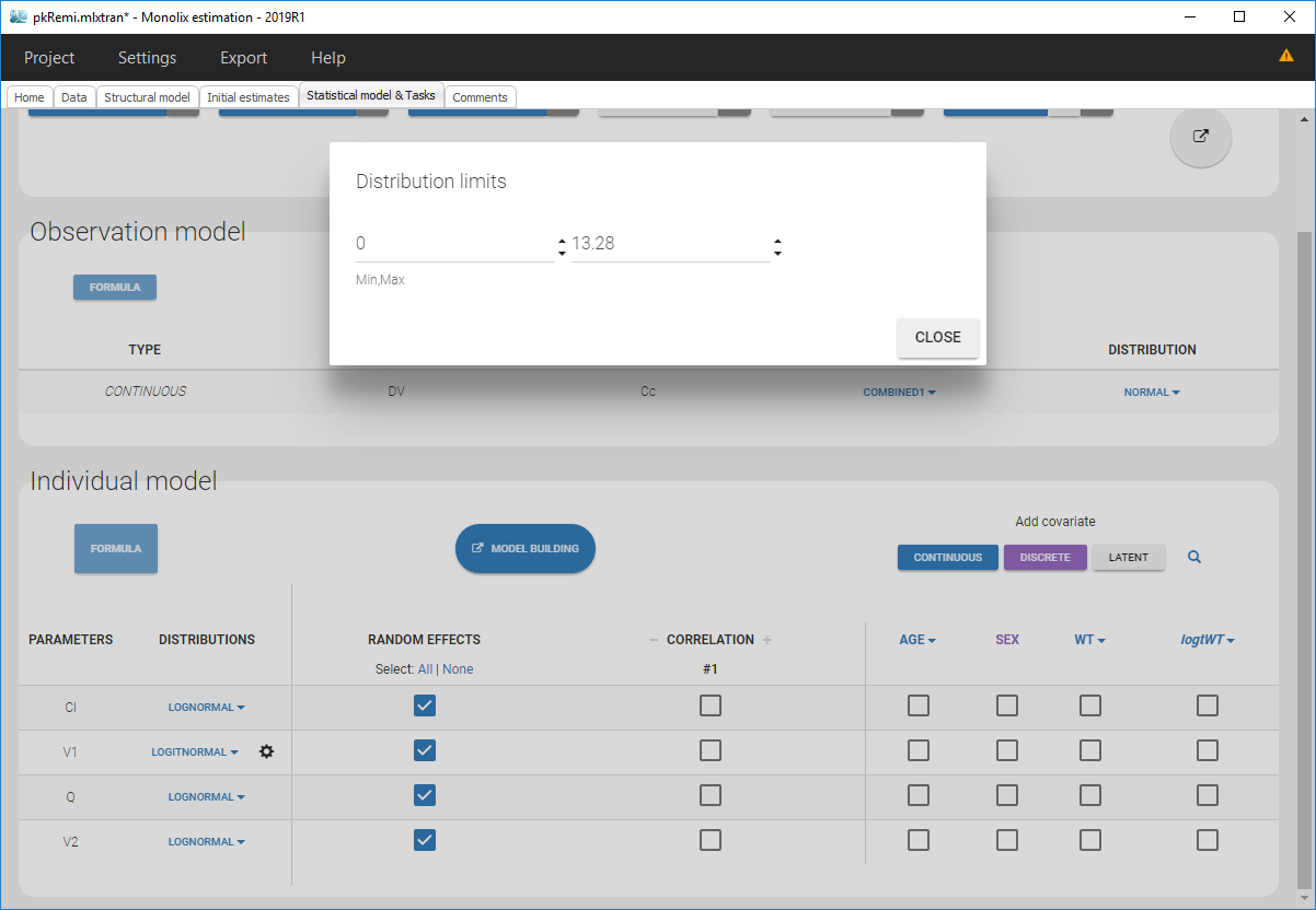
Notice that if your parameter initial value is not in [0, 1], the bounds are automatically adapted and the following warning message is proposed “The initial value of XX is greater than 1: the logit limit is adjusted”

Marginal distributions of the individual parameters

warfarin_distribution1_project (data = ‘warfarin_data.txt’, model = ‘lib:oral1_1cpt_TlagkaVCl.txt’)

We use the warfarin PK example here. The four PK parameters Tlag, ka, V and Cl are log-normally distributed. LOGNORMAL distribution is then used for these four log-normal distributions in the main Monolix graphical user interface:

The distribution of the 4 PK parameters defined in the MonolixGUI is automatically translated into Mlxtran in the project file:

[INDIVIDUAL]
input = {Tlag_pop, omega_Tlag, ka_pop, omega_ka, V_pop, omega_V, Cl_pop, omega_Cl}
DEFINITION:
Tlag = {distribution=lognormal, typical=Tlag_pop, sd=omega_Tlag}
ka = {distribution=lognormal, typical=ka_pop, sd=omega_ka}
V = {distribution=lognormal, typical=V_pop, sd=omega_V}
Cl = {distribution=lognormal, typical=Cl_pop, sd=omega_Cl}

Estimated parameters are the parameters of the 4 log-normal distributions and the parameters of the residual error model:

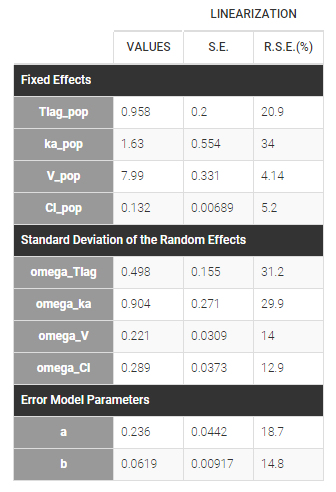
Here, $V_{\rm pop} = 7.94$ and $\omega_V=0.326$ means that the estimated population distribution for the volume is: $\log(V_i) \sim {\cal N}(\log(7.94) , 0.326^2)$ or, equivalently, $V_i = 7.94 e^{\eta_i}$ where $\eta_i \sim {\cal N}(0,0.326^2)$.

Remarks:

$V_{\rm pop} = 7.94$ is not the population mean of the distribution of $V_i$, but the median of this distribution (in that case, the mean value is 7.985). The four probability distribution functions are displayed figure Parameter distributions:
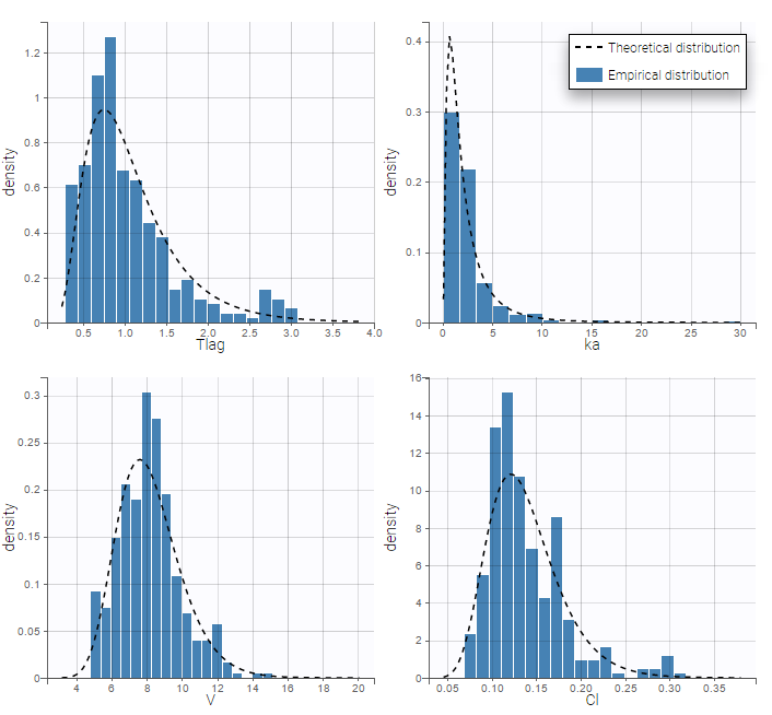
$V_{\rm pop}$ is not the population mean of the distribution of $V_i$, but the median of this distribution. The same property holds for the 3 other distributions which are not Gaussian.
Here, standard deviations $\omega_{Tlag}$, $\omega_{ka}$, $\omega_V$ and $\omega_{Cl}$ are approximately the coefficients of variation (CV) of Tlag, ka, V and Cl since these 4 parameters are log-normally distributed with variances < 1.

warfarin_distribution2_project (data = ‘warfarin_data.txt’, model = ‘lib:oral1_1cpt_TlagkaVCl.txt’)

Other distributions for the PK parameters are used in this project:

NORMAL for Tlag, we fix the population value $Tlag_{\text{pop}}$ to 1.5 and the standard deviation $\omega_{\rm Tlag}$ to 1:
NORMAL for ka,
NORMAL for V,
and LOGNORMAL for Cl

Estimated parameters are the parameters of the 4 transformed normal distributions and the parameters of the residual error model:

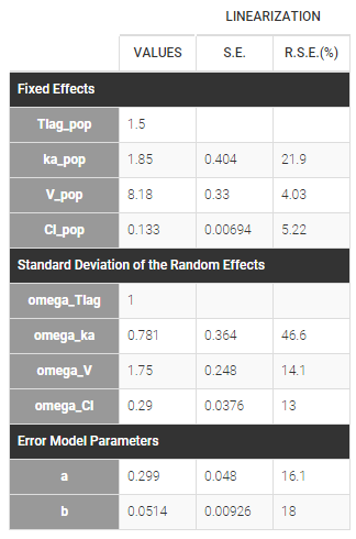
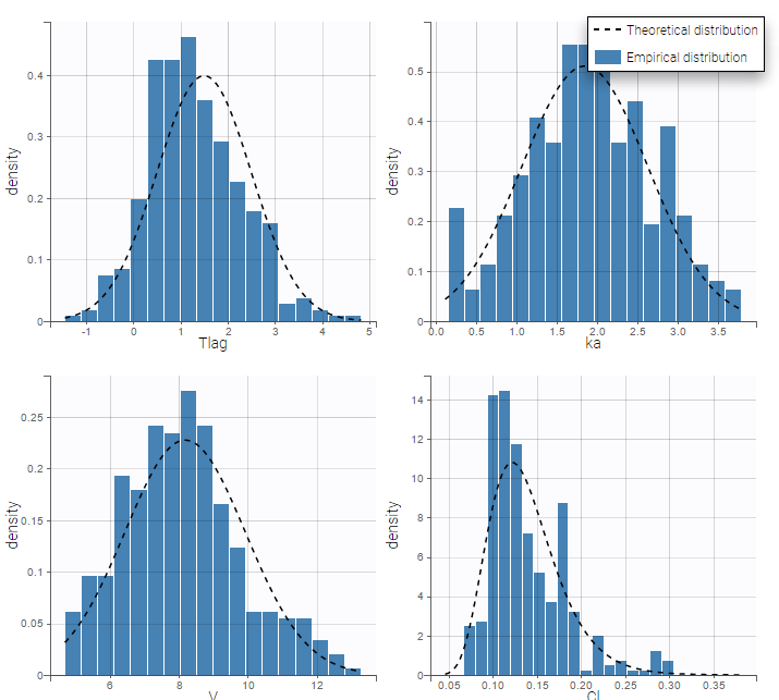
Here, $ Tlag_{\rm pop} = 1.5$ and $\omega_{Tlag}=1$ means that $Tlag_i \sim {\cal N}(1.5, 1^2)$ while $Cl_{\rm pop} = .133$ and $\omega_{Cl}=..29$ means that $log(Cl_i) \sim {\cal N}(log(.133), .29^2)$. The four probability distribution functions are displayed Figure Parameter distributions:

Correlation structure of the random effects

Dependency can be introduced between individual parameters by supposing that the random effects $\eta_i$ are not independent. This means considering them to be linearly correlated.

warfarin_distribution3_project (data = ‘warfarin_data.txt’, model = ‘lib:oral1_1cpt_TlagkaVCl.txt’)

Defining correlation between random effects in the interface

To introduce correlations between random effects in Monolix, one can define correlation groups. For example, two correlation groups are defined on the interface below, between $\eta_{V,i}$ and $\eta_{Cl,i}$ (#1 in that case) and between $\eta_{Tlag,i}$ and $\eta_{ka,i}$ in an other group (#2 in that case):

To define a correlation between the random effects of V and Cl, you just have to click on the check boxes of the correlation for those two parameters. If you want to define a correlation between the random effects ka and Tlag independently of the first correlation group, click on the + next to CORRELATION to define a second group and click on the check boxes corresponding to the parameters ka and Tlag under the correlation group #2. Notice, that as the random effects of Cl and V are already in the correlation group #1, these random effects can not be used in another correlation group. When three of more parameters are included in a correlation groups, all pairwise correlations will be estimated. It is not instance not possible to estimate the correlation between $\eta_{ka,i}$ and $\eta_{V,i}$ and between $\eta_{Cl,i}$ and $\eta_{V,i}$ but not between $\eta_{Cl,i}$ and $\eta_{ka,i}$.

It is important to mention that the estimated correlations are not the correlation between the individual parameters (between $Tlag_i$ and $ka_i$, and between $V_i$ and $Cl_i$) but the (linear) correlation between the random effects (between $\eta_{Tlag,i}$ and $\eta_{ka,i}$, and between $\eta_{V,i}$ and $\eta_{Cl,i}$ respectively).

Remarks

If the box is greyed, it means that the associated random effects can not be used in a correlation group, as in the following cases
- when the parameter has no random effects
- when the random effect of the parameter is already used in another correlation group
There are no limitation in terms of number of parameters in a correlation group
You can have a look in the FORMULA to have a recap of all correlations
In case of inter-occasion variability, you can define the correlation group for each level of variability independently.
The initial value for the correlations is zero and cannot be changed.
The correlation value cannot be fixed.

Estimated population parameters now include these 2 correlations:

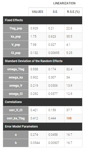
Notice that the high uncertainty on $\text{corr_ka_Tlag}$ suggests that the correlation between $\eta_{Tlag,i}$ and $\eta_{ka,i}$ is not reliable.

How to decide to include correlations between random effects?

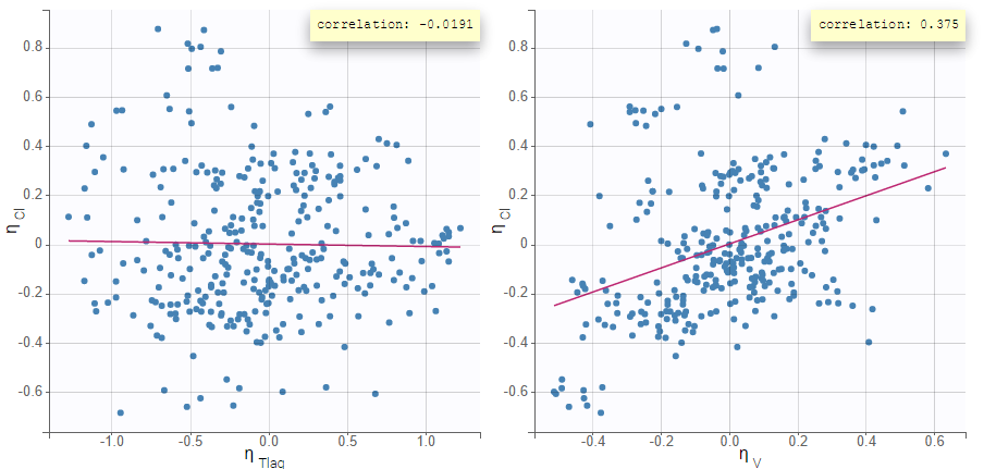
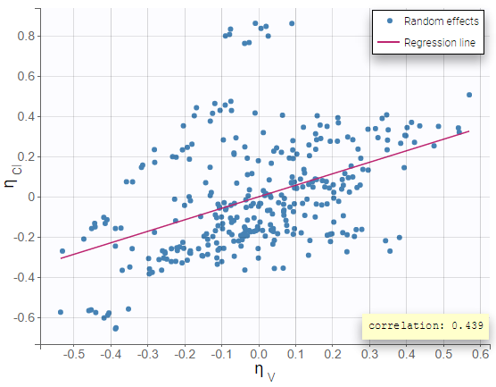
The scatterplots of the random effects can hint at correlations to include in the model. This plot represents the joint empirical distributions of each pair of random effects. The regression line (in pink below) and the correlation coefficient (“information” toggle in the settings) permits to visually detect tendencies. If “conditional distribution” (default) is chosen in the display settings, the displayed random effects are calculated using individual parameters sampled from the conditional distribution, which permits to avoid spurious correlations (see the page on shrinkage for more details). If a large correlation is present between a pair of random effects, this correlation can be added to the model in order to be estimated as a population parameter.

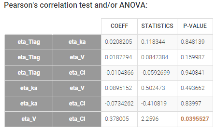
Depending on a number of random effects values used to calculate the correlation coefficient, a same correlation value can be more or less significant. To help the user identify significant correlations, Pearson’s correlation tests are performed in the “Result” tab, “Tests” section. If no significant correlation is found, like for the pair $\eta_{Tlag}$ and $\eta_{Cl}$ below, the distributions can be assumed to be independent. However, if a significant correlation appears, like for the pair $\eta_V$ and $\eta_{Cl}$ below, it can be hypothesized that the distributions are not independent and that the correlation must be included in the model and estimated. Once the correlation is included in the model, the random effects for $V$ and $Cl$ are drawn from the joint distribution rather than from two independent distributions.

How do the correlations between random effects affect the individual model?

In this example the model has four parameters Tlag, ka, V and Cl. Without correlation, the individual model is:
$log(Tlag) = log(Tlag_{pop}) + \eta_{Tlag}$
$log(ka) = log(ka_{pop}) + \eta_{ka}$
$log(V) = log(V_{pop}) + \eta_V$
$log(Cl) = log(Cl_{pop}) + \eta_{Cl}$

The random effects follow normal distributions: $(\eta_{Tlag,i},\eta_{ka,i},\eta_{V,i},\eta_{Cl,i}) \sim \mathcal{N}(0,\Omega)$
$\Omega$ is the variance-covariance matrix defining the distributions of the vectors of random effects, here:

$\Omega = \begin{pmatrix} \omega_{Tlag}^2 & 0 & 0 & 0 \\ 0 & \omega_{ka}^2 & 0 & 0 \\ 0 & 0 & \omega_V^2 & 0 \\ 0 & 0 & 0 & \omega_{Cl}^2 \end{pmatrix}$

In this example, two correlations between $\eta_{Tlag}$ and $\eta_{ka}$ and between $\eta_{V}$ and $\eta_{Cl}$ are added to the model. They are defined with two population parameters called $\text{corr_Tlag_ka}$ and $\text{corr_V_Cl}$ that appear in the variance-covariance matrix. So the only difference in the individual model is in $\Omega$, that is now:

$\Omega = \begin{pmatrix} \omega_{Tlag}^2 & \omega_{Tlag} \omega_{ka} \text{corr_Tlag_ka} & 0 & 0 \\ \omega_{Tlag} \omega_{ka} \text{corr_Tlag_ka} & \omega_{ka}^2 & 0 & 0 \\ 0 & 0 & \omega_V^2 & \omega_{V} \omega_{Cl} \text{corr_V_Cl} \\ 0 & 0 & \omega_{V} \omega_{Cl} \text{corr_V_Cl} & \omega_{Cl}^2 \end{pmatrix}$

So the correlation matrix is related to the variance-covariance matrix $\Omega$ as:

$$\text{corr}(\theta_i,\theta_j)=\frac{\text{covar}(\theta_i,\theta_j)}{\sqrt{\text{var}(\theta_i)}\sqrt{\text{var}(\theta_j)}}$$

Why should the correlation be estimated as part of the population parameters?

The effect of correlations is especially important when simulating parameters from the model. This is the case in the VPC or when simulating new individuals in Simulx to assess the outcome of a different dosing scenario for instance. If in reality individuals with a large distribution volume also have a large clearance (i.e there is a positive correlation between the random effects of the volume and the clearance), but this correlation has not been included in the model, then the concentrations predicted by the model for a new cohort of individuals will display a larger variability than they would in reality.

How do the EBEs change after having included correlation in the model?

Before adding correlation in the model, the EBEs or the individual parameters sampled from the conditional distribution may already be correlated, as can be seen in the “correlation between random effects” plot. This is because the individual parameters (EBEs or sampled) are based on the individual conditional distributions, which takes into account the information given by the data. Especially when the data is rich, the data can indicate that individuals with a large volume of distribution also have a large clearance, even if this correlation is not yet included in the model.

Including the correlation in the model as a population parameter to estimate allows to precisely estimate its value. Usually, one can see a stronger correlation for the corresponding pair of random effects when the correlation is included in the model compared to when it is not. In this example, after including the correlations in the individual model, the joint distribution of $\eta_{V}$ and $\eta_{Cl}$ displays a higher correlation coefficient (0.439 compared to 0.375 previously):

warfarin_distribution4_project (data = ‘warfarin_data.txt’, model = ‘lib:oral1_1cpt_TlagkaVCl.txt’)

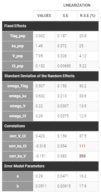
In this example, $Tlag_i$ does not vary in the population, which means that $\eta_{Tlag,i}=0$ for all subjects i, while the three other random effects are correlated:

Estimated population parameters now include the 3 correlations between $\eta_{ka,i}$, $\eta_{V,i}$ and $\eta_{Cl,i}$ :

Parameters without random effects

Adding/removing inter-individual variability

By default, all parameters have inter-individual variability. To remove it, click on the checkbox of the random effect column:

How the parameters with no variability are estimated is explained here.

Custom parameter distributions

Some datasets may require more complex parameter distributions that those pre-implemented in the Monolix GUI. This video shows how to implement a lognormal distribution with Box-Cox transformation and how to bound a parameter between two values using a transformed logit distribution (this latter case can be handled automatically from Monolix2019R1).

Distribution of the individual parameters