Several statistical tests may be automatically performed to test the different components of the model. These tests use individual parameters drawn from the conditional distribution, which means that you need to run the task “Conditional distribution” in order to get these results. In addition, the tests for the residuals require to have first generated the residuals diagnostic plots (scatter plot or distribution).
The tests are all performed using the individual parameters sampled from the conditional distribution (or the random effects and residuals derived thereof). They are thus not subject to bias in case of shrinkage. For each individual, several samples from the conditional distribution may be used. The used tests include a correction to take into account that these samples are correlated among each other.
Results of the tests are available in the tab “Results” and selecting “Tests” in the left menu
The model for the individual parameters
Consider a PK example (warfarin data set from the demos) with the following model for the individual PK parameters (ka, V, Cl):

In this example, the different assumptions we make about the model are:
- The 3 parameters are lognormally distributed
- ka is function of sex
- V is function of sex and weight. More precisely, the log-volume log(V) is a linear function of the log-weight \({\rm lw70 }= \log({\rm wt}/70)\).
- Cl is not function of any of the covariates.
- The random effects \(\eta_V\) and \(\eta_{Cl}\) are linearly correlated
- \(\eta_{ka}\) is not correlated with \(\eta_V\) and \(\eta_{Cl}\)
Let’s see how each of these assumptions are tested:
Covariate model
Individual parameters vs covariates – Test whether covariates should be removed from the model
If an individual parameter is function of a continuous covariate, the linear correlation between the transformed parameter and the covariate is not 0 and the associated \(\beta\) coefficient is not 0 either. To detect covariates bringing redundant information, we check if these beta coefficients are different from 0. For this, we perform two different tests: a correlation test based on betas coefficients estimated with a linear regression, and a Wald test relying on the estimated population parameters and their standard error.
In both cases, a small p-value indicates that the null hypothesis can be rejected and thus that the estimated beta parameter is significantly different from zero. If this is the case, the covariate should be kept in the model. On the opposite, if the p-value is large, the null hypothesis cannot be rejected and this suggests to remove the covariate from the model. Note that if beta is equal to zero, then the covariate has no impact on the parameter. High p-values are colored in yellow (p-value in [0.01-0.05]), orange (p-value in [0.05-0.10]) or red (p-value in [0.10-1]) to draw attention on parameter-covariate relationships that can be removed from the model from a statistical point of view.
Correlation test
Briefly, we perform a linear regression between the covariates and the transformed parameters and test if the resulting beta coefficient are different from 0.
More precisely: for each individual \(i\), let \(z_i^l\) be the transformed individual parameters (e.g log(V) for log-normally distributed parameters or logit(F) for logit-distributed parameters) sampled from the conditional distribution (called replicates, index l). Here we will call covariates all continuous covariates and all non-referent categories of categorical covariates \(cov^{(c)}, c = 1..n_C\). For each individual \(i\), \(cov_i^{(c)}\) is the value of the c\(^{th}\) covariate, equal to 0 or 1 if the covariate is a category.
The transformed individual parameters are first averaged over replicates for each individual:
$$z_i^{(L)}=\frac{1}{L} \sum_{l=1}^{L} z_i^l$$
We then perform the following linear regression:
$$z_i^{(L)}=\alpha_0 + \sum_{c=1}^{n_c} \beta_c \text{cov}_i^{(c)} + e_i$$
If two covariates \(cov^{(1)}\) and \(cov^{(2)}\) (for example WT and BMI) are strongly correlated with a parameter \(z^{(L)}\) (for example the volume), only one of them is needed in the model because they are redundant. In the linear regression, only one of the estimated \(\hat{\beta_1}\) and \(\hat{\beta_2}\) will be significantly different from zero.
For each covariate \(c\) we conduct a t-test on the \(\hat{\beta_c}\) with the null hypothesis:
H0: \(\beta_c = 0\).
The test statistic is
$$T_0 = \frac{\hat{\beta_c}}{se(\hat{\beta_c})}$$
where \(se(\hat{\beta_c})\) is the estimated standard error of \(\hat{\beta_c}\) (obtained by least squares estimation during the regression). If the null hypothesis is true, \(T_0\) follows a t distribution with \(N-n_C-1\) degrees of freedom (where N is the number of individuals).
In our example, the correlation test suggests to remove sex from ka:

Wald test
The Wald test relies on the standard errors. Thus the task “Standard errors” must have been calculated to see the test results. The test can be performed using the standard errors calculated using either the “linearization method” (indicated as “linearization”) or not (indicated as “stochastic approximation” in the tests).
The Wald test tests the following null hypothesis:
H0: the beta parameter estimated by SAEM is equal to zero.
The math behind: Let’s note \( \hat{\beta} \) the estimated beta value (which is a population parameter) and \(se(\hat{\beta}) \) the associated standard error calculated during the task “Standard errors”. The Wald test statistic is:
$$W=\frac{\hat{\beta}}{se(\hat{\beta})} $$
The test statistic is compared to a normal distribution (z distribution).
In our example, the Wald test suggests to remove sex from ka and V:

Remark: the Wald test and the correlation test may suggest different covariates to keep or remove. Note that the null hypothesis tested is not the same.
Random effects vs covariates – Test whether covariates should be added to the model
Pearson’s correlation tests and ANOVA are performed to check if some relationships between random effects and covariates not yet included in the model should be added to the model.
For continuous covariates, the Pearson’s correlation test tests the following null hypothesis:
H0: the person correlation coefficient between the random effects (calculated from the individual parameters sampled from the conditional distribution) and the covariate values is zero
For categorical covariates, the one-way ANOVA tests the following null-hypothesis:
H0: the mean of the random effects (calculated from the individual parameters sampled from the conditional distribution) is the same for each category of the categorical covariate
A small p-value indicates that the null hypothesis can be rejected and thus that the correlation between the random effects and the covariate values is significant. If this is the case, it is probably worth considering to add the covariate in the model. Note that the decision of adding a covariate in the model should not only be driven by statistical considerations but also biological relevance. Note also that for parameter-covariate relationships already included in the model, the correlation between the random effects and covariates is not significant (while the correlation between the parameter and the covariate can be – see above). Small p-values are colored in yellow (p-value in [0.05-0.10]), orange (p-value in [0.01-0.05]) or red (p-value in [0.00-0.01]) to draw attention on parameter-covariate relationships that can be considered for addition in the model from a statistical point of view.
In our example, we already have sex on ka and V, and lw70 on V in the model. The only remaining relationship that could possibly be worth investigating is between weight (or the log-transformed weight “lw70”) and clearance.

The math behind:
Continuous covariate: Let \(\eta_i^l\) the random effects corresponding to the \(L\) individual parameters sampled from the conditional distribution (called replicates) for individual \(i\), and \(cov_i\) the covariate value for individual \(i\). The random effects are first averaged over replicates for each individual:
$$ \eta_i^{(L)}=\frac{1}{L} \sum_{l=1}^{L} \eta_i^l $$
We note \(\overline{cov} = \sum_{i=1}^N cov_i \) the average covariate value over the N subjects and \(\overline{\eta}=\sum_{i=1}^N \eta_i^{(L)} \) the average random effect. The Pearson correlation coefficient is calculated as:
$$r=\frac{\sum_{i=1}^N(cov_i – \overline{cov})(\eta_i^{(L)} – \overline{\eta})}{\sqrt{ \sum_{i=1}^N(cov_i – \overline{cov})^2 \sum_{i=1}^N(\eta_i^{(L)} – \overline{\eta})^2}}$$
The test statistic is:
$$t=\frac{r}{\sqrt{1-r^2}}\sqrt{N-2}$$
and it is compared to a t-distribution with \(N-2\) degrees of freedom with \(N\) the number of individuals.
Categorical covariates: The random effects are first averaged over replicates for each individual and a one-way analysis of variance is performed (simplified to a t-test when the covariate has only two categories).
The model for the random effects
Distribution of the random effects – Test if the random effects are normally distributed
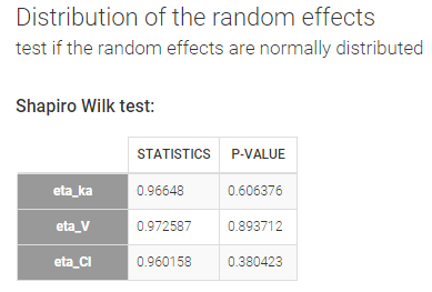
In the individual model, the distributions for the parameters assume that the random effects follow a normal distribution. Shapiro-Wilk tests are performed to test this hypothesis. The null hypothesis is:
H0: the random effects are normally distributed
If the p-value is small, there is evidence that the random effects are not normally distributed and this calls the choice of the individual model (parameter distribution and covariates) into question. Small p-values are colored in yellow (p-value in [0.05-0.10]), orange (p-value in [0.01-0.05]) or red (p-value in [0.00-0.01]).
In our example, there is no reason to reject the null-hypothesis and no reason to question the chosen log-normal distributions for the parameters.
The math behind: Let \(\eta_i^l\) the random effects corresponding to the \(L\) individual parameters sampled from the conditional distribution (called replicates) for individual \(i\). The Shapiro-Wilk test statistic is calculated for each replicate \(l\) (i.e the first sample from all individuals, then the second sample from all individuals, etc):
$$W^l=\frac{\left( \sum_{i=1}^N a_i \eta_i^l \right)^2}{ \sum_{i=1}^N (\eta_i^l – \overline{\eta}^l)^2}$$
with \(a_i\) tabulated coefficient and \(\overline{\eta}^l=\frac{1}{N}\sum_{i=1}^N \eta_i^l \) the average over all individuals, for each replicate.
The statistic displayed in Monolix corresponds to the average statistic over all replicates \(W=\frac{1}{L}\sum_{l=1}^L W^l \). For the p-values, one p-value is calculated for each replicate, using the Shapiro-Wild table with \(N\) (number of individuals) degrees of freedom. The Benjamini-Hochberg (BH) procedure is then applied: the p-values are ranked by ascending order and the BH critical value is calculated for each as \( \frac{\textrm{rank}}{L}Q \) with \(\textrm{rank}\) the individual p-value’s rank, \(L\) the total number of p-values (equal to the number of replicates) and \(Q=0.05\) the false discovery rate. The largest p-value that is smaller than the corresponding critical value is selected.
Joint distribution of the random effects – Test if the random effects are correlated
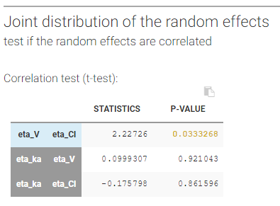
Correlation tests are performed to test if the random effects (calculated from the individual parameters sampled from the conditional distribution) are correlated. The null-hypothesis is:
H0: the expectation of the product of the random effects of the first and second parameter is zero
The null-hypothesis is assessed using a t-test.
Remark: In the 2018 version, a Pearson correlation test was used.
For correlations not yet included in the model, a small p-value indicates that there is a significant correlation between the random effects of two parameters and that this correlation should be estimated as part of the model (otherwise simulations from the model will assume that the random effects of the two parameters are not correlated, which is not what is observed for the random effects estimated using the data). Small p-values are colored in yellow (p-value in [0.05-0.10]), orange (p-value in [0.01-0.05]) or red (p-value in [0.00-0.01]).
For correlations already included in the model, a large p-value indicates that one cannot reject the hypothesis that the correlation between the random effects is zero. If the correlation is not significantly different from zero, it may not be worth estimating it in the model. High p-values are colored in yellow (p-value in [0.01-0.05]), orange (p-value in [0.05-0.10]) or red (p-value in [0.10-1])
In our example, we have assumed in the model that \(\eta_V\) and \(\eta_{Cl}\) are correlated. The high p-value (0.033, above the 0.01 threshold, see above) indicates that the correlation between the random effects of V and Cl is not significantly different from zero and suggests to remove this correlation from the model.
Remark: as correlations can only be estimated by groups (i.e if a correlation is estimated between (ka, V) and between (V, Cl), then one must also estimate the correlation between (ka, Cl)), it may happen that it is not possible to remove a non-significant correlation without removing also a significant one.
The math behind: Let \(\eta_{\psi_1,i}^l\) and \(\eta_{\psi_2,i}^l\) the random effects corresponding to the \(L\) individual parameters \(\psi_1\) and \(\psi_2\) sampled from the conditional distribution (called replicates) for individual \(i\). First we calculate the product of the random effects averaged over the replicates:
$$p_i^{(L)} = \frac{1}{L} \sum_{l=1}^{L} \eta_{\psi_1,i}^l \eta_{\psi_2,i}^l $$
We note \( \overline{p}=\sum_{i=1}^{N} p_i^{(L)} \) the average of the product over the individuals and \(s\) their standard deviation. The test statistic is:
$$ T=\frac{\overline{p}}{\frac{s}{\sqrt{N}}}$$
and it is compared to a t-distribution with \(N-1\) degrees of freedom with \(N\) the number of individuals.
The distribution of the individual parameters
Distribution of the individual parameters not dependent on covariates – Test if transformed individual parameters are normally distributed
When an individual parameter doesn’t depend on covariates, its distribution (normal, lognormal, logit or probit) can be transformed into the normal distribution. Then, a Shapiro-Wilk test can be used to test the normality of the transformed parameter. The null hypothesis is:
H0: the transformed individual parameter values (sampled from the conditional distribution) is normally distributed
If the p-value is small, there is evidence that the transformed individual parameter values are not normally distributed and this calls the choice of the parameter distribution into question. Small p-values are colored in yellow (p-value in [0.05-0.10]), orange (p-value in [0.01-0.05]) or red (p-value in [0.00-0.01]).
In our example, there is no reason to reject the null hypothesis of lognormality for Cl.

Remark: testing the normality of a transformed individual parameter that does not depend on covariates is equivalent to testing the normality of the associated random effect. We can check in our example that the Shapiro-Wilk tests for \(\log(Cl)\) and \(\eta_{Cl}\) are equivalent.
The math behind: Let \(z_i^l\) the transformed individual parameters (e.g log(V) for log-normally distributed parameters and logit(F) for logit-distributed parameters) sampled from the conditional distribution (called replicates, index \(l\) ) for individual \(i\). The Shapiro-Wilk test statistic is calculated for each replicate \(l\) (i.e the first sample from all individuals, then the second sample from all individuals, etc):
$$W^l=\frac{\left( \sum_{i=1}^N a_i z_i^l \right)^2}{ \sum_{i=1}^N (z_i^l – \overline{z}^l)^2}$$
with \(a_i\) tabulated coefficient and \(\overline{z}^l=\frac{1}{N}\sum_{i=1}^N z_i^l \) the average over all individuals, for each replicate.
The statistic displayed in Monolix corresponds to the average statistic over all replicates \(W=\frac{1}{L}\sum_{l=1}^L W^l \). For the p-values, one p-value is calculated for each replicate, using the Shapiro-Wild table with \(N\) (number of individuals) degrees of freedom. The Benjamini-Hochberg (BH) procedure is then applied: the p-values are ranked by ascending order and the BH critical value is calculated for each as \( \frac{\textrm{rank}}{L}Q \) with \(\textrm{rank}\) the individual p-value’s rank, \(L\) the total number of p-values (equal to the number of replicates) and \(Q=0.05\) the false discovery rate. The largest p-value that is smaller than the corresponding critical value is selected.
Distribution of the individual parameters dependent on covariates – test the marginal distribution of each individual parameter
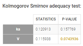
Individual parameters that depend on covariates are not anymore identically distributed. Each transformed individual parameter is normally distributed, with its own mean that depends on the value of the individual covariate. In other words, the distribution of an individual parameter is a mixture of (transformed) normal distributions. A Kolmogorov-Smirnov test is used for testing the distributional adequacy of these individual parameters. The null-hypothesis is:
H0: the individual parameters are samples from the mixture of transformed normal distributions (defined by the population parameters and the covariate values)
A small p-value indicates that the null hypothesis can be rejected. Small p-values are colored in yellow (p-value in [0.05-0.10]), orange (p-value in [0.01-0.05]) or red (p-value in [0.00-0.01]).
With our example, we obtain:
The model for the observations
A combined1 error model with a normal distribution is assumed in our example:

Distribution of the residuals
Several tests are performed for the individual residuals (IWRES), the NPDE and for the population residuals (PWRES).
Test if the distribution of the residuals is symmetrical around 0
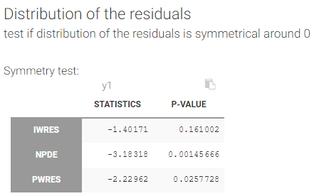
A Miao, Gel and Gastwirth (2006) test (or Van Der Waerden test in the 2018 release) is used to test the symmetry of the residuals. Indeed, symmetry of the residuals around 0 is an important property that deserves to be tested, in order to decide, for instance, if some transformation of the observations should be done. The null hypothesis tested is:
H0: the median of the residuals is equal to its mean
A small p-value indicates that the null hypothesis can be rejected. Small p-values are colored in yellow (p-value in [0.05-0.10]), orange (p-value in [0.01-0.05]) or red (p-value in [0.00-0.01]).
With our example, we obtain:
The math behind: Let \(R_i\) the residuals (NPDE, PWRES or IWRES) for each individual \(i\), \(\overline{R}\) the mean of the residuals, and \(M_R\) their median. The MGG test statistic is:
$$T=\frac{\sqrt{n}}{0.9468922}\frac{\overline{R}-M_R}{ \sum_{i=1}^{n}|R_i-M|}$$
with \(n\) the number of residuals. The test statistic is compared to a standard normal distribution.
The formula above is valid for i.i.d (independent and identically distributed) residuals. For the IWRES, the residuals corresponding to a given time and given id are not independent (they ressemble each other). To solve the problem, we estimate an effective number of residuals. The number of residuals \(n\) can be split into the number of replicates \(L\) times the number of observations \(m\). We look for the effective number of replicates \(\tilde{L}\) such that:
$$ \frac{\tilde{L}}{L} \sum_{l=1}^L (R_i^l)^2 \approx \chi^2(\tilde{L})$$
using a maximum likelihood estimation. The number of residuals is then calculated as \(n=\tilde{L} \times m \).
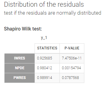
Test if the residuals are normally distributed
A Shapiro Wilk test is used for testing the normality of the residuals. The null hypothesis is:
H0: the residuals are normally distributed
If the p-value is small, there is evidence that the residuals are not normally distributed. The Shapiro Wilk test is known to be very powerful. Then, a small deviation of the empirical distribution from the normal distribution may lead to a very significant test (i.e. a very small p-value), which does not necessarily means that the model should be rejected. Thus, no color highlight is made for this test.
In our example, we obtain:
The math behind: Let \(R_i^l\) the residuals (NPDE, PWRES or IWRES) for individual \(i\). NPDE and PWRES have one values per time points and per individual. IWRES have one value per time point, per individual and per replicate (corresponding to the \(L\) individual parameters sampled from the conditional distribution). The Shapiro-Wilk test statistic is calculated for each replicate \(l\) (i.e the first sample from all individuals, then the second sample from all individuals, etc):
$$W^l=\frac{\left( \sum_{i=1}^N a_i R_i^l \right)^2}{ \sum_{i=1}^N (R_i^l – \overline{R}^l)^2}$$
with \(a_i\) tabulated coefficient and \(\overline{R}^l=\frac{1}{N}\sum_{i=1}^N R_i^l \) the average over all individuals, for each replicate.
The statistic displayed in Monolix corresponds to the average statistic over all replicates \(W=\frac{1}{L}\sum_{l=1}^L W^l \). For the p-values, one p-value is calculated for each replicate, using the Shapiro-Wild table with \(N\) (number of individuals) degrees of freedom. The Benjamini-Hochberg (BH) procedure is then applied: the p-values are ranked by ascending order and the BH critical value is calculated for each as \( \frac{\textrm{rank}}{L}Q \) with \(\textrm{rank}\) the individual p-value’s rank, \(L\) the total number of p-values (equal to the number of replicates) and \(Q=0.05\) the false discovery rate. The largest p-value that is smaller than the corresponding critical value is selected.
