Download data set only | Download Monolix and Simulx project files | Download simulx R script
This case study is a detailed modeling and simulation workflow on a TTE data set. We recommended to read before the Introduction to TTE data and library of models in Monolix.
A second case study on time-to-event data is also available: Case study on NCCTG lung cancer data set
In this case study, we develop a model for the survival of patients with advanced lung cancer. We show how to investigate the effect of several covariates, including a novel chemotherapy, and then use the final model to simulate new scenarios.
Introduction
The following study has been conducted by the US Veterans Administration. It contains male patients with advanced inoperable lung cancer who received either a standard therapy or a test chemotherapy. Time to death was recorded for 137 patients, while 9 left the study before death. The study includes also various covariates for each patient.
The primary goal is to assess if the test chemotherapy is beneficial. Secondary goals include the analysis of covariates as prognostic variables.
This data set has been initially presented and analyzed in:
Data set visualization
The data set includes data for 137 patients, 9 of them are right censored. According to the data set formatting guidelines, the data set includes for each patient a line indicating the start time (time = 0 and observation Y = 0), and a line indicating either the time of death (Y = 1) or the time at which the patient has left the study (Y = 0).
In addition the following covariates were recorded:
- Treatment (“trt” column): “standard” or “test” (tested new chemotherapy)
- Histological type of the tumor (“celltype” column): “squamous”, “smallcell”, “adeno” or “large”
- Karnofsky score (“karno” column): performance score that describes the overall patients status at the beginning of the study. The scale goes from 0 (dead) to 100 (completely healthy). More details about the scale can be found here.
- Time between diagnosis and start of the study (column “diagtime”): in months
- Age (column “age”): in years
- Prior therapy (column “priortherapy”): indicates if the patient has received another therapy before the current one
A snapshot of the data set in shown below:

We start with a visualization of the data set in Monolix: open Monolix, click on New project and Browse the data set. The figure below show the columns tagging (the covariates must be assigned to CONTINUOUS COVARIATE for continuous covariates or CATEGORICAL COVARIATE for categorical covariates):
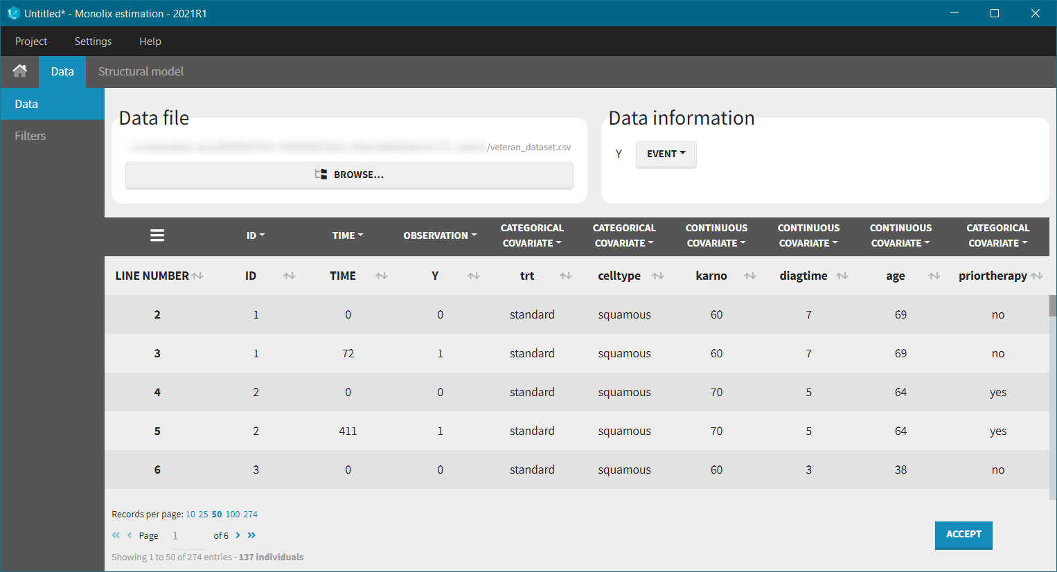
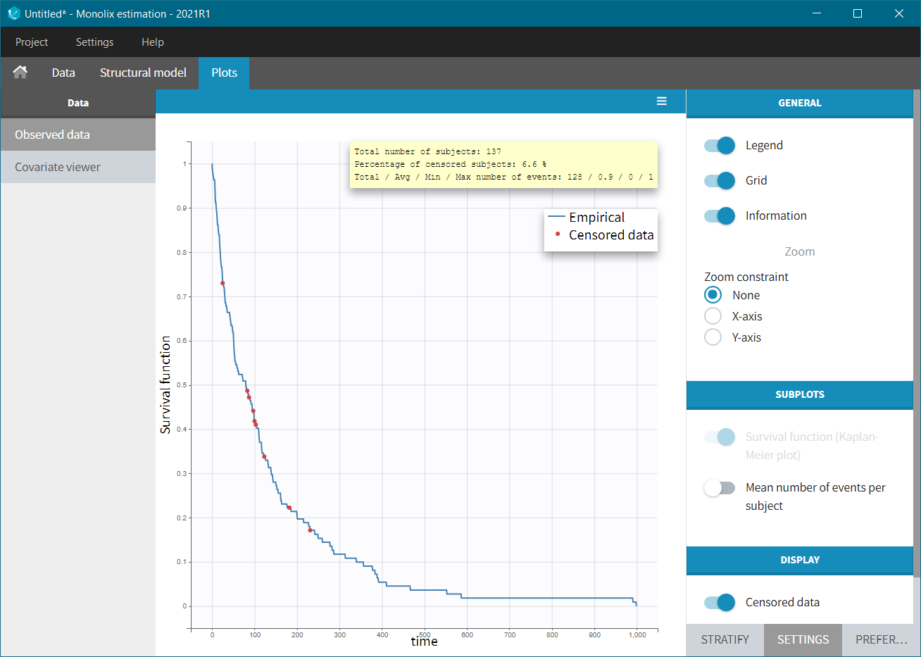
Before “Accepting” the dataset, we must indicate that the data is of type TTE (rather than continuous) – “Data information” section Y:EVENT. We can now accept the column assignments by clicking on “ACCEPT” button. A new tab “Plots” appear, where we can visualized the TTE data: the Kaplan-Meier (KM) estimate of the survival curve and the mean number of events curve (SUBPLOTS). Censored data are marked in red in the KM survival curve, and can be removed from the DISPLAY settings.
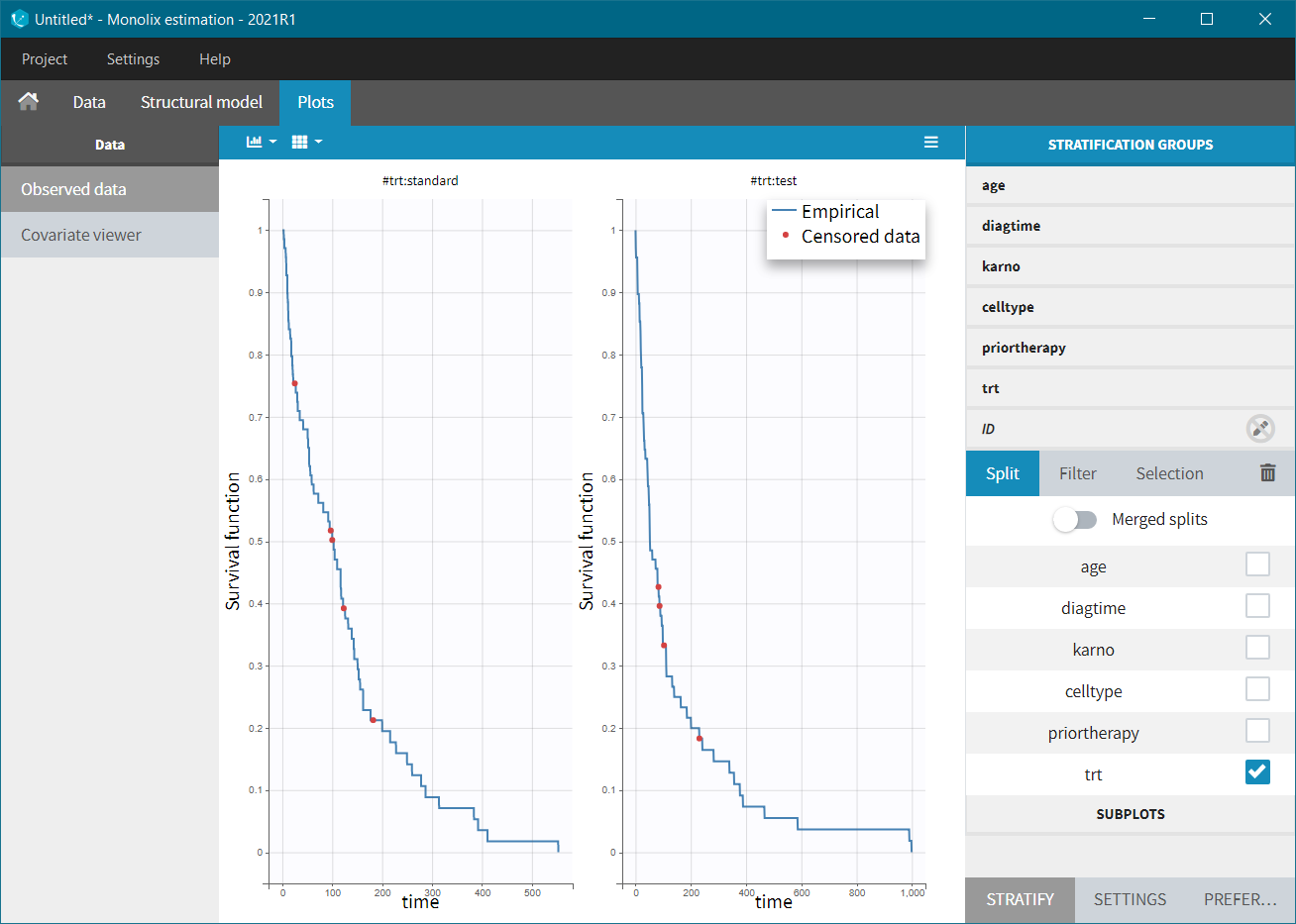
In the Stratification panel, we can split a KM curve according to categorical and continuous covariates (or stratification covariates) and then “merge” the plots in one figure with different colors (fixed) for each curve. Use the legend to show the information about the colors assignment. Stratifying by treatment “trt” (and using the “merge” option) leads to the following figure:
 |
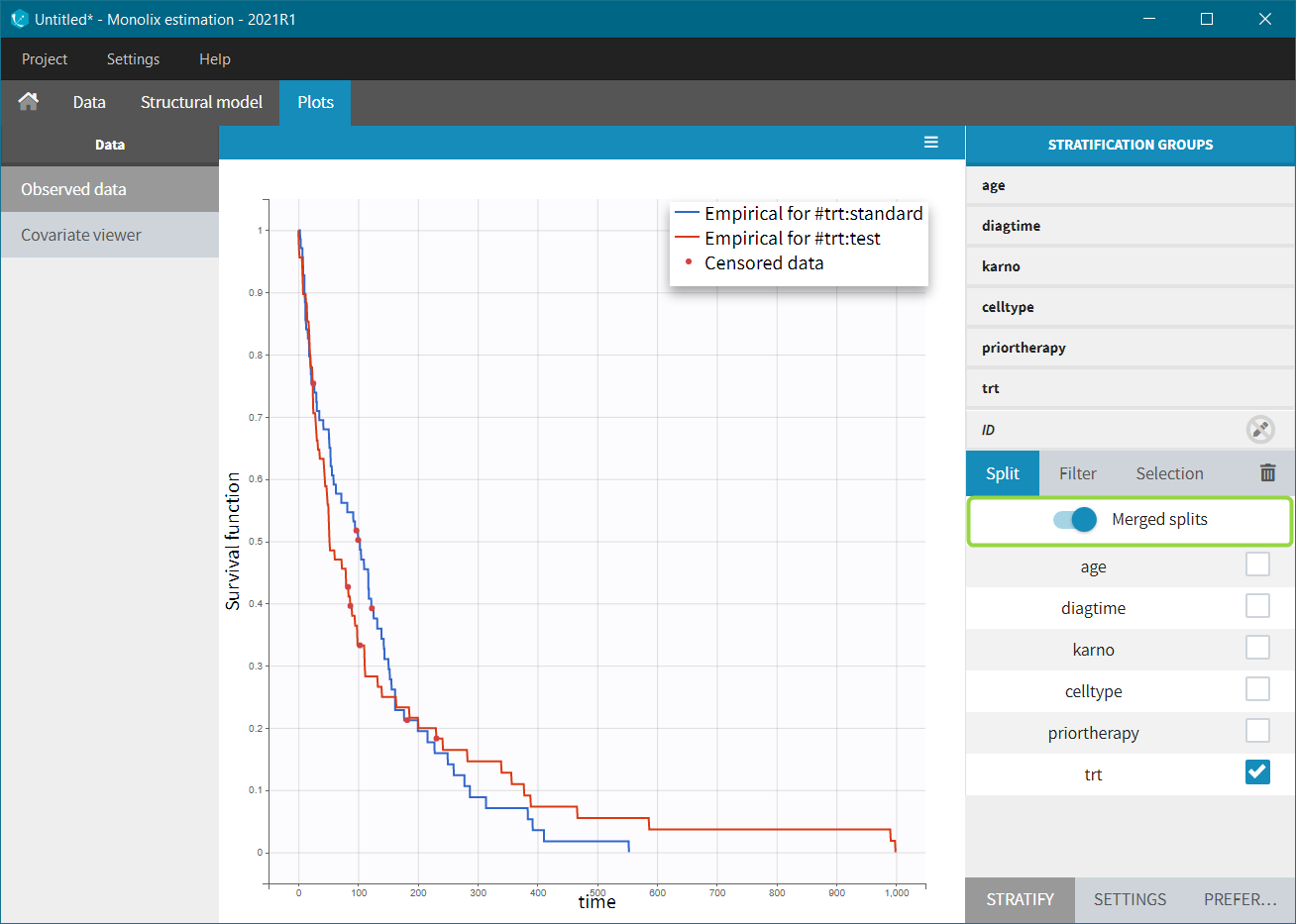 |
It does not show a significant difference in survival between the standard treatment group and the chemotherapy treatment group. Stratification using the Karnofsky score in two groups (Group1 = karno<50, and Group2 = karno>50) gives:
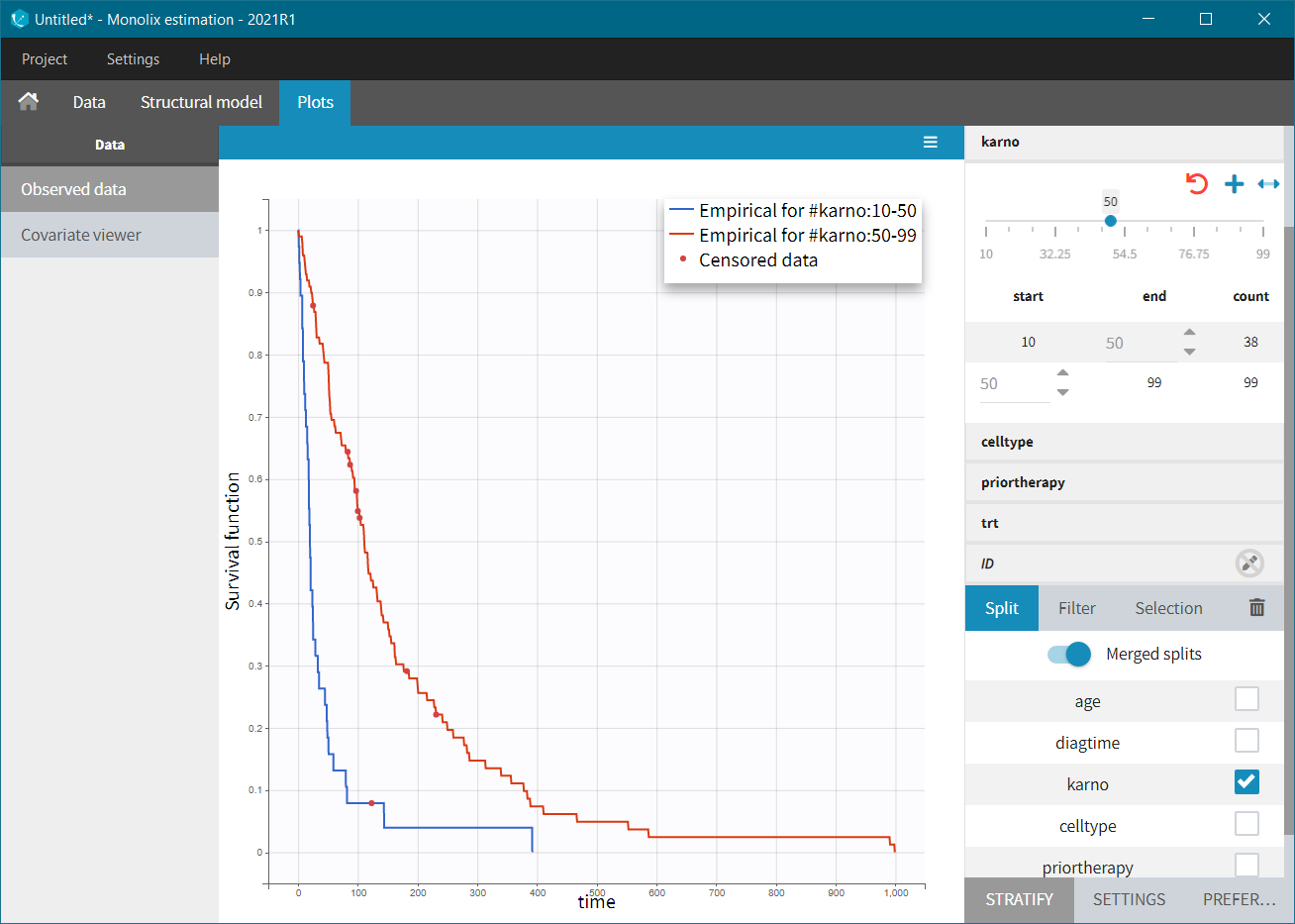
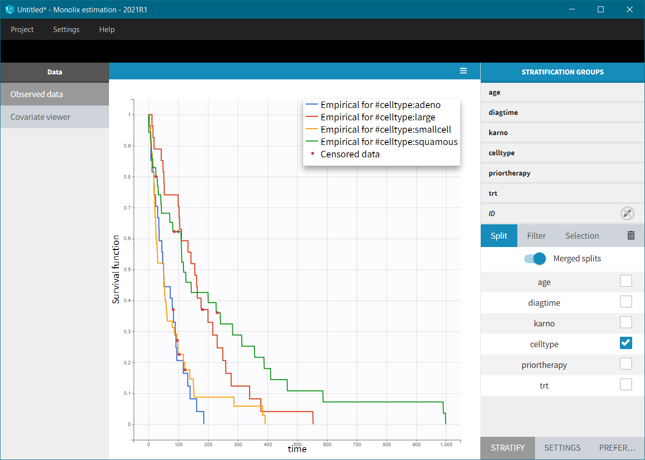
Here, we observed that patients with higher Karnofsky score (higher general health status) have a tendency to survive longer. The histological type of a tumur “celltype” also has an impact on the survival curve. It seems that squamous and large cells types are less malignous and those patients survive longer.
Note also that the survival curves for “adeno” and “small cell” types are very similar, so for comparison, these two groups could be joined together (drag&drop method in the stratification group).
Modeling with Monolix
Now we are going to develop a model for this data set and analyze the influence of the covariates, in particular the treatment. Within the MonolixSuite, the model must be fully specified via its hazard function (no non-parametric or semi-parametric approaches).
Structural model
We start with the specification of the structural model. In the TTE introduction, you will find a description of the library of common TTE models (defined via their hazard functions), and presentation of typical shapes of the resulting survival curve. Based on the visualization of the data, the Kaplan-Meier curve, and using the overview of the library models presented in the TTE introduction, the exponential model seems appropriate. We thus choose from the library the model file “exponential_model_singleEvent.txt” with a single event type because death happens only once per individual.
Next we define the distribution of the individual parameters.
- Most of the time in survival analysis, one assumes that the individual parameters are influenced by the covariates and all individuals with the same covariates have the same individual parameters – thus the same hazard function (but different times of death).
- On the opposite, we can also assume a random effect for the individual parameters (often called frailty models). It permits to capture heterogeneity between individuals, which cannot be explained by the covariates.
Monolix estimation algorithms and plots are most powerful when parameters include random effects, so we will start with this latter approach.
The model contains a single parameter, the characteristic time Te. This parameter should remain positive, so we keep the default log-normal distribution. An initial value for this parameter can be chosen with the help of the library overview, for instance 100 for this data set. Starting from the 2021R1 version of the MonolixSuite, the AUTO-INIT is available also for time-to-even models.

When a model is defined, we can launch the estimation tasks: estimation of the population parameters, estimation of the standard errors via the Fisher Information Matrix, estimation of the log-likelihood and generation of the plots (individual parameters have been skipped because no individual fits plots are possible with TTE data). The Te_pop parameter converges rapidly towards a random walk around the maximum likelihood estimate (MLE) in the exploratory phase of SAEM (before the red line, see figure below), and then converges to the MLE in the smoothing phase (after the red line). The estimated value (visible in the Results tab) is 109, close to our initial estimate. The standard deviation of the random effects (omega_Te parameter) converges to 0.63, which corresponds to a coefficient of variation of \( \textrm{CV} = \sqrt{e^{{\omega_{T_e}}^2} – 1} = 50 % \). The large inter-individual variability probably means that sub-populations within the data set have different Te values. In the next section we will consider adding covariates to the Te parameter to explain this variability and to reduce the random effects.

To assess if the exponential model was a good choice, we can display the VPC for Time-to-Event data (click on the list icon next to the task Plots and in the pop-up window, on “Visual Predictive Check”; starting from the 2021R1 this plot is generated automatically by default). The figure displays the empirical Kaplan-Meier curve overlayed with the 90% prediction interval calculated from model simulations. The figure is then interpreted similarly to a VPC, see here for more details how this plot is generated. In this example, the empirical Kaplan-Meier curve lies within the prediction interval, which indicates no model mis-specification.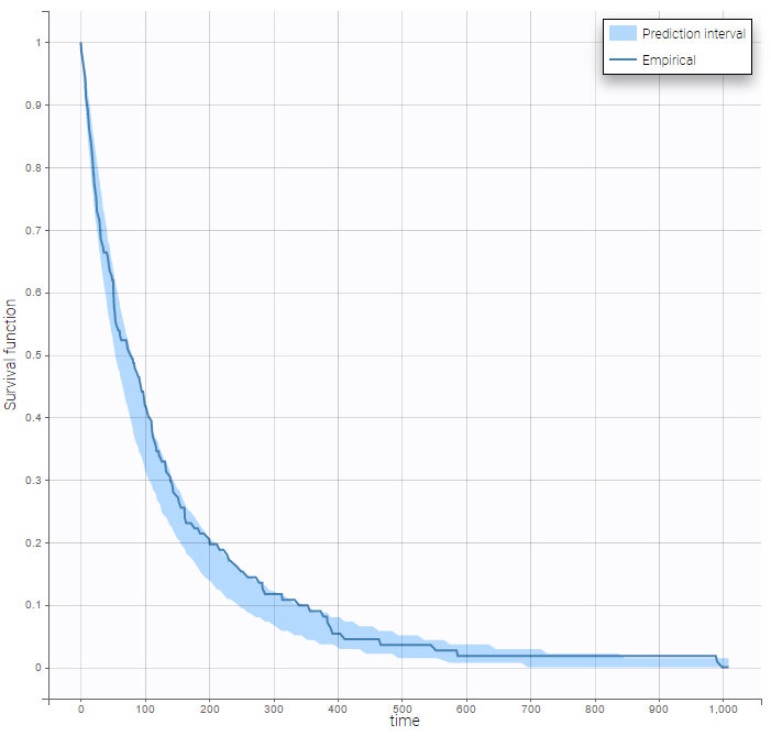
Covariate search
The next step is to assess if the hazard is significantly different for sub-populations (for instance with the standard treatment or the chemotherapy). For model selection several statistical tools can be used, such as information criteria (AIC and BIC) or hypothesis tests (Wald test and likelihood ratio test). In this case study, we will use the Wald test.
Covariates can be added by clicking on the boxes in the “Individual model” section:
 The details of the resulting equations can be seen by clicking on the “f(x)” icon. If we add the categorical covariate trt on parameter Te, we obtain:
$$T_{e,i} = \begin{cases} T_{e,\textrm{pop}}e^{\eta_i} & \text{if} \quad \textrm{trt}=0\textrm{ (reference)} \\ T_{e,\textrm{pop}}e^{\beta_{\textrm{trt}}}e^{\eta_i} & \text{if} \quad \textrm{trt}=1 \end{cases} $$
If we instead add the continuous covariate karno on parameter Te, we obtain:
$$T_{e,i}=T_{e,\textrm{pop}}e^{\beta_{\textrm{karno}}\times\textrm{karno}}e^{\eta_i}$$
Note that this parameterization corresponds to the typical form of a Cox proportional model. Via transformation of the covariates, other forms are also possible.
The parameterization using betas permits to directly perform statistical tests on the beta parameters. In particular, the Wald test tests the following null hypothesis:
$$H_0:\quad \textrm{”}\beta=0\textrm{”} \quad \textrm{versus} \quad H_1:\quad \textrm{”}\beta\neq 0\textrm{”}$$
The associated p-value is reported in Results tab in the Tests section – the Standard errors task must be run. If the p-value is smaller than a threshold (usually 0.05), we can consider that the corresponding \(\beta\) is significantly different from zero.
We create 8 models, each having one covariate on the Te parameter. Here are the p-value results for each covariate (each model):
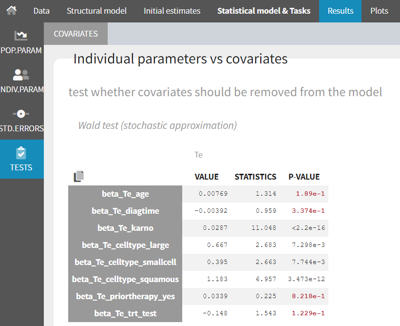
The covariates karno and celltype appear as significant, while all others not. In particular, given the data, the new chemotherapy does not significantly lower the risk, compared to the standard treatment.
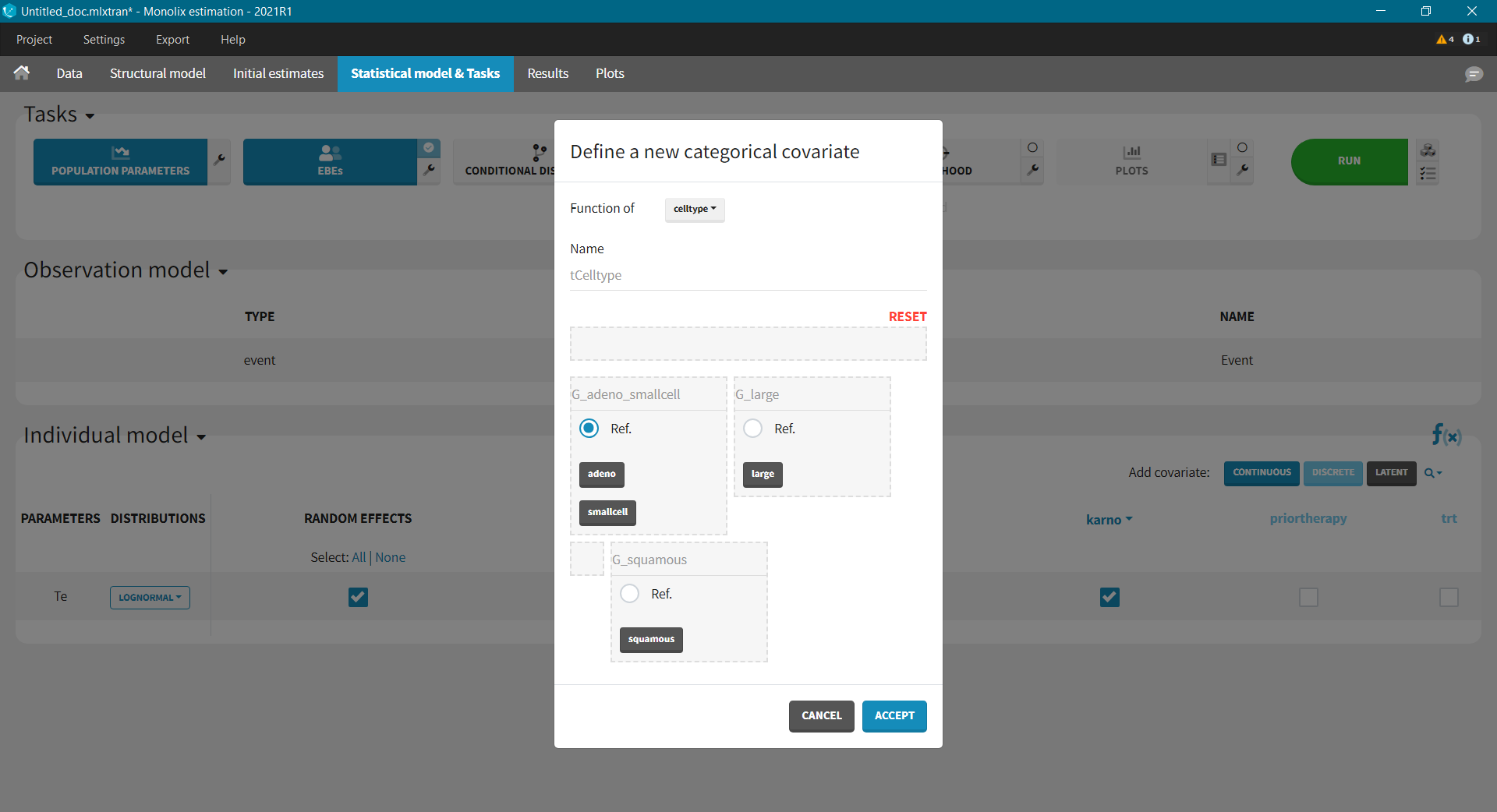
Next, we can try a model with both karno and celltype. Because the difference between the “smallcell” cell type and the “adeno” cell type (used as reference) is not significant (seen in the observed data plot), we can choose to group these two into one category. Add covariate: using the “Discrete” button, we create a new categorical covariate, where “adeno” and “smallcell” are put into the G1 reference group.
The results are the following:
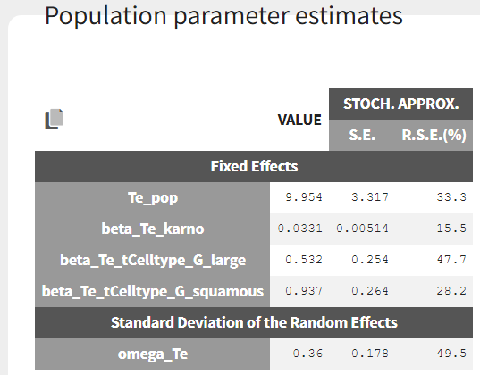
From the estimated beta values, we can easily calculate that the risk of death is around exp(0.937) = 2.6 times higher for patients with squamous cell types, compared to adeno or small cell types. In the graphics, the 95% prediction interval for the survival can be stratified by cell type and/or karno score categories, to verify the agreement between model and data: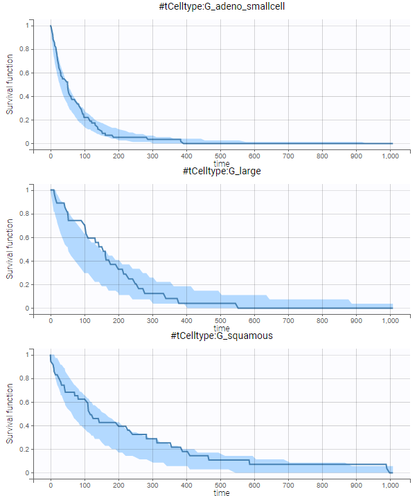
No model mis-specification can be detected. We thus consider this model as our final model.
The final model is:
$$h_{i}(t)=\begin{cases} \frac{1}{T_{e,\textrm{pop, adeno/smallcell}}e^{\beta\times \textrm{karno}}e^{\eta_i} }& \text{if} \quad \textrm{celltype}=\textrm{adeno or smallcell (G_adeno_smallcell)} \\ \frac{1}{T_{e,textrm{pop, large}}e^{\beta\times \textrm{karno}}e^{\eta_i} }& \text{if} \quad \textrm{celltype}=\textrm{large (G_large)}\\ \frac{1}{T_{e,\textrm{pop, squamous}}e^{\beta\times \textrm{karno}}e^{\eta_i}} & \text{if} \quad \textrm{celltype}=\textrm{squamous (G_squamous )} \end{cases} $$
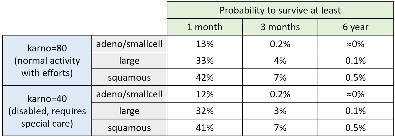
For a given cell type and a given karno score, we can easily calculate analytically the typical hazard and the associated exponential model survival (i.e if \(h(t)=\lambda\) then \(S(t)=e^{-\lambda t})\). From the survival function, we calculate the probability to survive at least 1 month (30 days), 3 months (90 days) or 6 months (180 days), depending on the cell type and karno score:
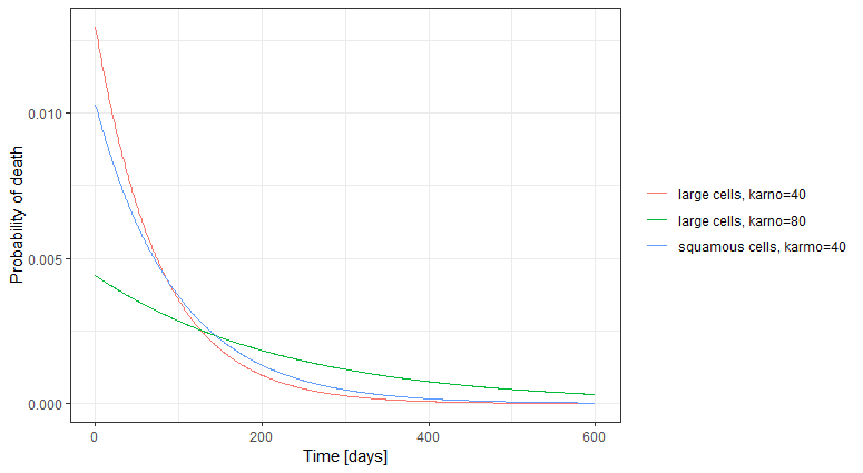
The probability density function of the death event can also be calculated for any given karno score and cell type ( \( f(t)=h(t)*S(t) \) ), giving the probability of death over time. For each displayed subpopulation, the plot also represents the distribution of death times in the subpopulation.
Simulations using Simulx
We have developed a parametric model for the survival of patients with advanced lung cancer. Now we can use it to explore the expected survival for new cohorts of patients. To perform simulations, we use the Simulx application. The Monolix project can be directly exported to Simulx (Menu/Export/Save and export to Simulx) and used as an input, to either simulate the same population as in the original data set, or to define new populations.
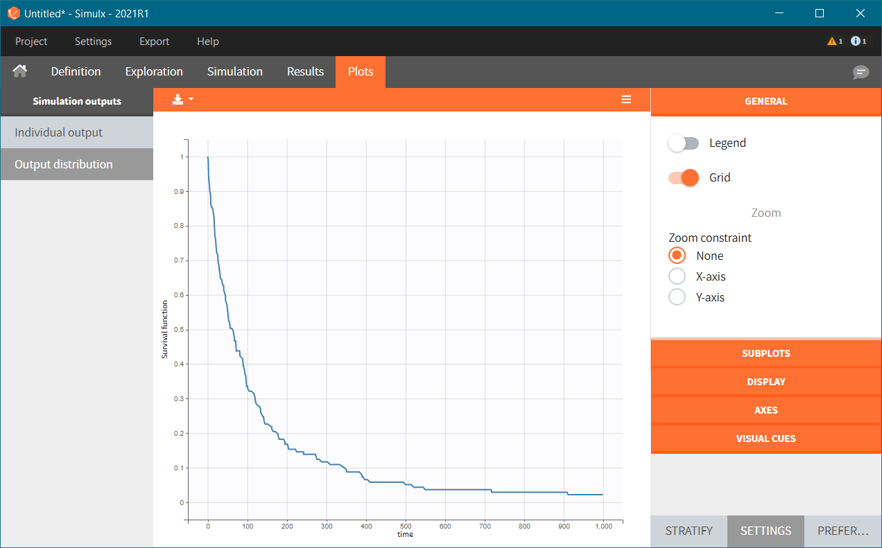
We first simulate the same population as in the original data set. After exporting the Monolix project to Simulx, the simulation scenario in the Simulation tab is set to re-simulate the originl dataset.
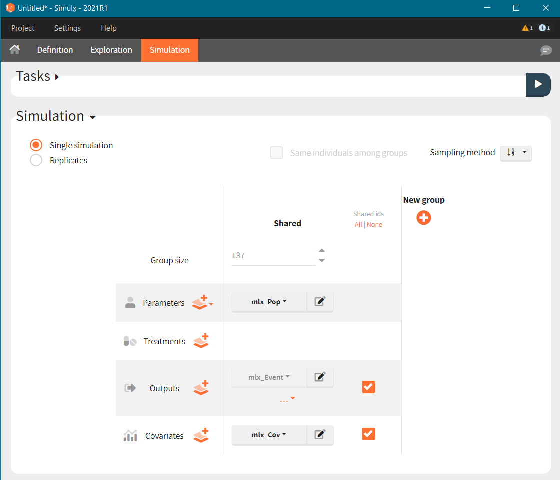
For a given hazard, time of death is a random variable, so the re-simulated Kaplan-Meier survival curve is different compared to the original data.
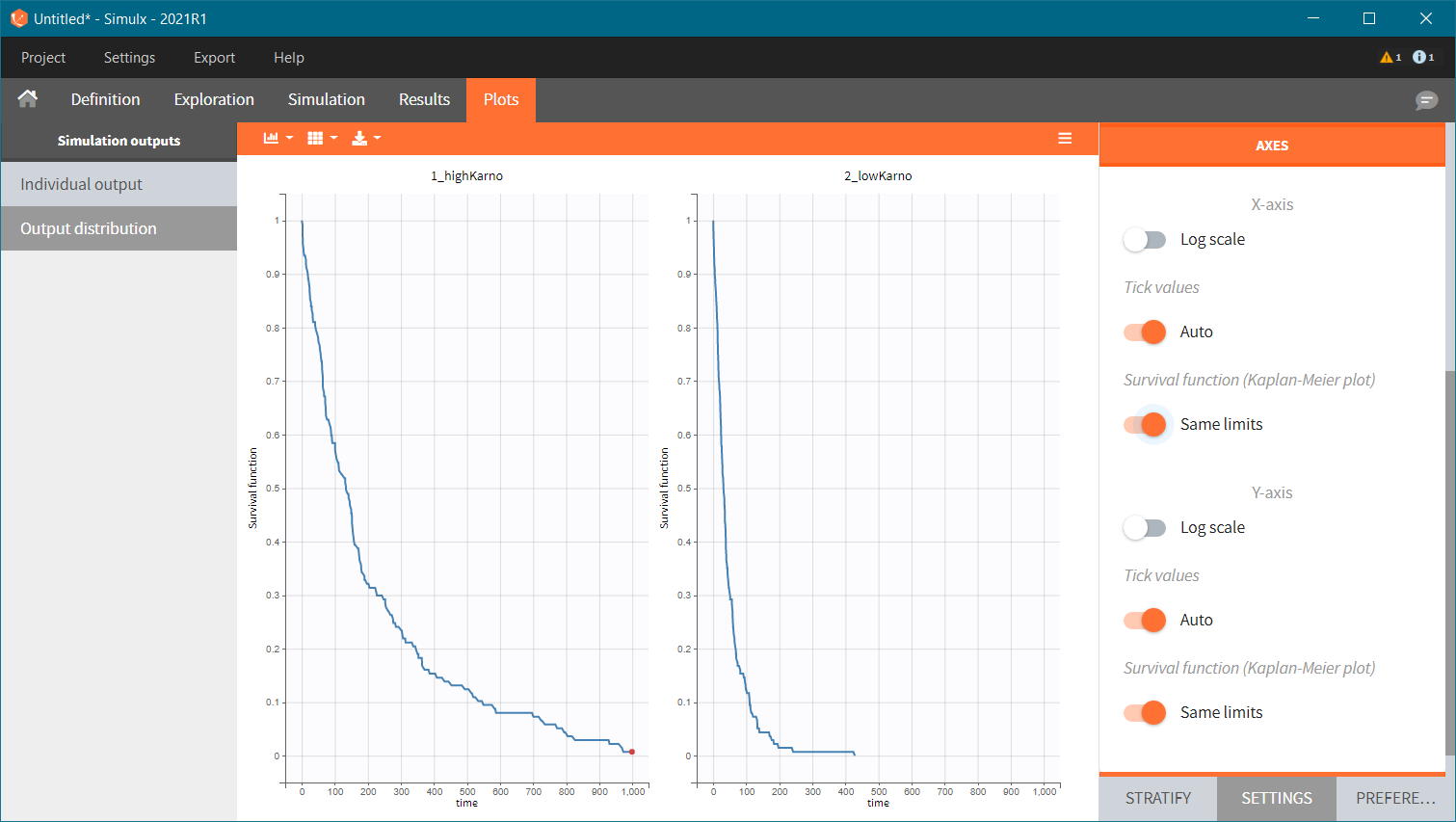
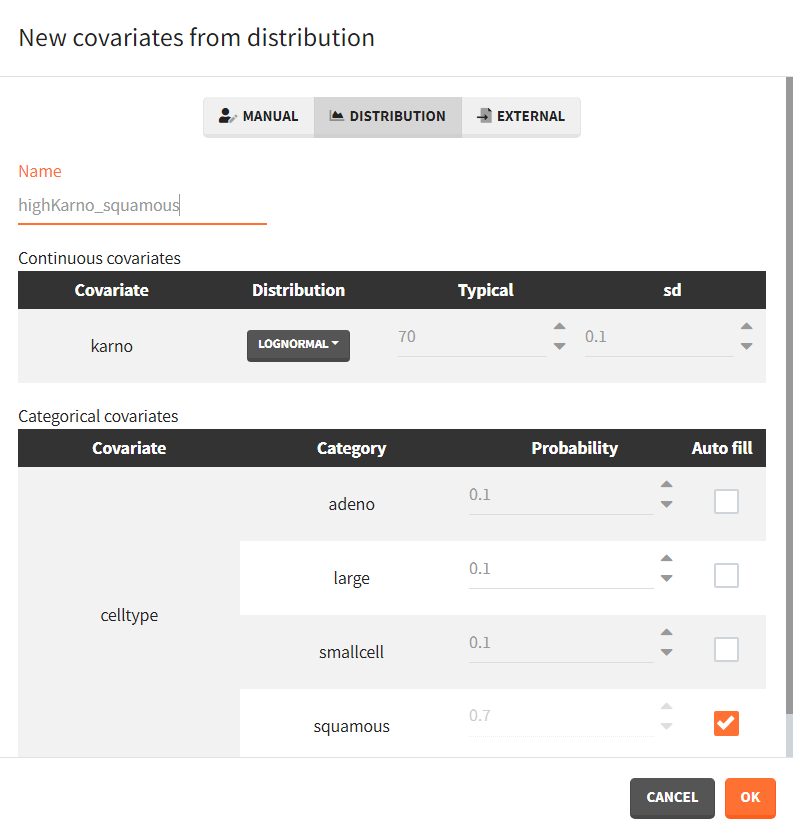
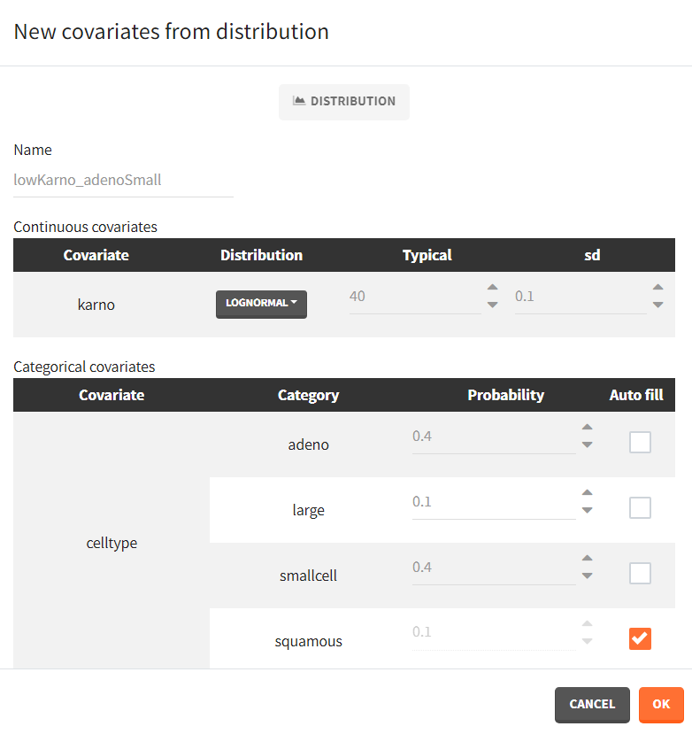
We next simulate two new patients cohorts (with different covariates compared to the original data set). The first cohort is composed of patients with a quite good karno score, around 70, and mostly with squamous cell types (70% squamous, 10% adeno, 10% smallcell, 10% large). The second cohort contains patients having mostly adeno or smallcell celltypes (40% adeno, 40% smallcell, 10% large, 10% squamous) and a low karno score, around 40. The two corresponding covariate elements are defined in Simulx with distributions:
 |
 |
To simulate these two cohorts, we create two groups in the simulation scenario, each using the same population parameters (mlx_pop) and the same observation time (mlx_Event), but with different covariates for individuals.
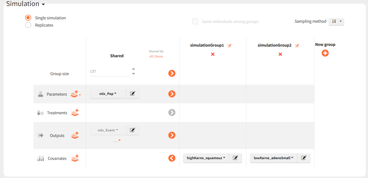
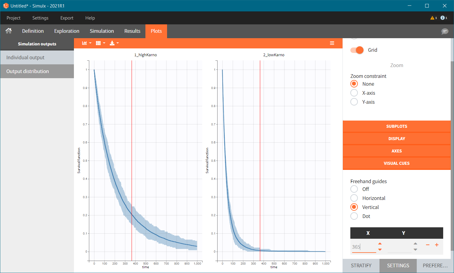
The Kaplan-Meier survival curves obtained in these two groups are:
Because the time of death is a random variable, several simulations of the same population will lead to different survival curves. We can assess the uncertainty of the survival curve by doing replicates. This can be done very easily by using Replicates instead of a single simulation. In the figure below, the blue line corresponds to the median Kaplan-Meier curve calculated over replicates and the shaded area is the 90% prediction interval. Visual clues can be added to compare different points in the plots – here a 1 year survival.
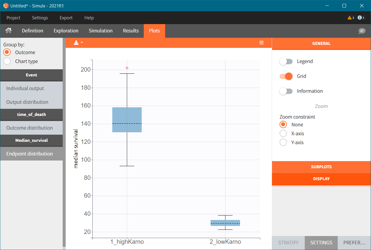
To quantitatively compare the median survival we use the post-processing tool in Simulx: outcomes & endpoints. It allows to calculate the median time of event (death) in each group, and asses the uncertainty due to the variability between individuals (when simulating replicates). The results are presented as a boxplot for the endpoint and in the results tables.
Simulations using RsSimulx function
The documentation on the RsSimulx R-function can be found here: https://simulx.lixoft.com/rssimulx/
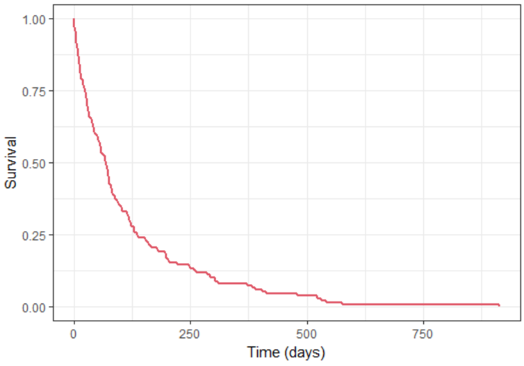
Re-simulate the original dataset. The simulation is done via the simulx function which returns an R object containing the result of the simulation (time of death for each individual). We use this object in the kmplotmlx function to obtain the Kaplan-meier survival curve:
# loading the RsSimulx library
library(RsSimulx)

# defining the path to the mlxtran project file
project.file <- "./monolixproject/project_veteran_3_celltype_karno.mlxtran"

# calling simulx, giving the path to the project as argument
res <- simulx(project = project.file)

# plotting the KM survival curve
kmplotmlx(res$Event) + xlab("Time (days)")
We obtain the following Kaplan-Meier survival curve, similar (but different) from that of the original data set:
We next simulate two new patients cohorts (with different covariates compared to the original data set). The first cohort is composed of patients with a quite good karno score, around 70, and mostly with squamous cell types (70% squamous, 10% adeno, 10% smallcell, 10% large). The second cohort contains patients having mostly adeno or smallcell celltypes (40% adeno, 40% smallcell, 10% large, 10% squamous) and a low karno score, around 40.
To simulate these two cohorts, we create two groups, each defined via a data frame of the individuals covariates, and pass them as simulx input argument. For instance for group 1:
# covariate data frame for group 1, with column id and one column per covariate
cov1 <- data.frame(id=1:137,
                   karno = rnorm(137,mean=70, sd=5),
                   celltype = c(rep("squamous",100),rep("large",12),rep("smallcell",12),rep("adeno",13)),
                   diagtime = NaN,                                #unused in model but must be present
                   age = NaN,                                     #unused in model but must be present
                   trt = c(rep("test",100),rep("standard",37)),   #unused in model but must be present
                   priortherapy = c(rep("yes",100),rep("no",37))) #unused in model but must be present

#============= calling simulx for group 1
res1 <- simulx(project = project.file,
               parameter = cov1)
After having put together the results for group 1 and group 2, we obtain the following prediction:
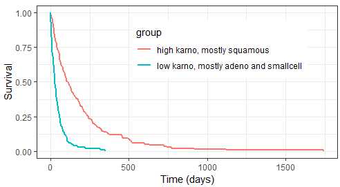
Because the time of death is a random variable, several simulations of the same population will lead to different survival curves. We can assess the uncertainty of the survival curve by doing replicates. This can be done very easily by adding an argument nrep:
res1 <- simulx(project = project.file,
               parameter = cov1,
               nrep = 100)
We then obtain a prediction interval for the two survival curves: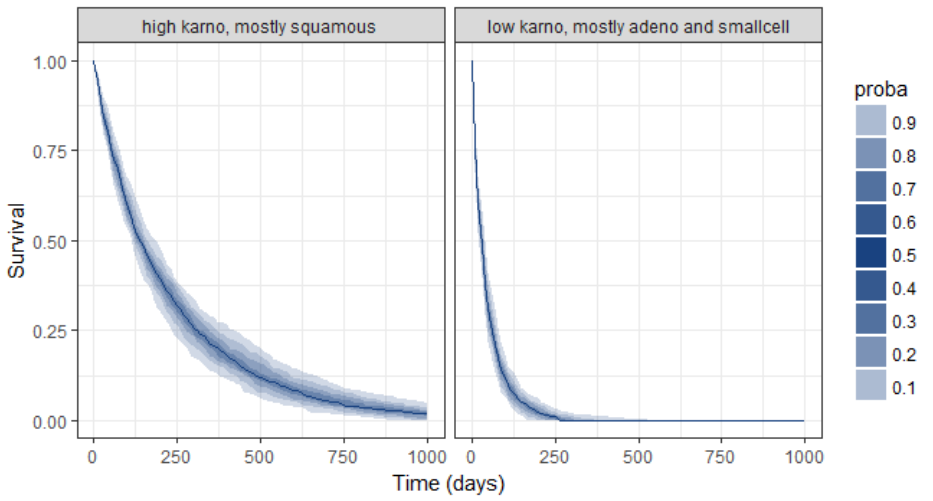
Conclusion
Monolix permits an efficient parametric analysis of this TTE data set. The risk of death for male patients with advanced inoperable lung cancer appears to be constant over time (exponential distribution of death times). Prognostic factors are the histological type of the tumor (cell type) and the overall health Karnofsky score. Unfortunately, no improvement with the new treatment can be shown, given the data. The parametric nature of the model permits to easily predict the survival probability for a typical subject with a given celltype and a given karno score.
Using Simulx, the developed parametric model can be used for more advanced predictions. Indeed, we can define new populations with a complex mix of covariates (different celltypes and different karno scores) and simulate the expected survival for this population. The uncertainty of the prediction can easily be assessed via replicates.
