Libraries of models

• The PK library
• The PD and PKPD libraries 
• The PK double absorption library
• The TMDD library
• The TTE library
• The Count library
• The TGI library
• A step-by-step example with the PK library

---

Objectives: learn how to use the Monolix libraries of models and use your own models.

---

Projects: theophylline_project, PDsim_project, warfarinPK_project, TMDD_project, LungCancer_project, hcv_project

---

For the definition of the structural model, the user can either select a model from the available model libraries or write a model itself using the Mlxtran language.
Discover how to easily choose a model from the libraries via step-by-step selection of its characteristics. An enriched PK, a PD, a joint PKPD, a target-mediated drug disposition (TMDD), and a time to-event (TTE) library are now available.

---

---

Model libraries

Five different model libraries are available in Monolix, which we will detail below. To use a model from the libraries, in the Structural model tab, click on Load from library and select the desired library. A list of model files appear, as well as a menu to filter them.  Use the filters and indications in the file name (parameters names) to select the model file you need.

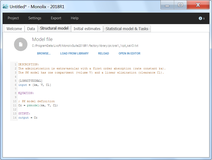
The model files are simply text files that contain pre-written models in Mlxtran language. Once selected, the model appears in the Monolix GUI. Below we show the content of the (ka,V,Cl) model:

The PK library

• theophylline_project (data = ‘theophylline_data.txt’ , model=’lib:oral1_1cpt_kaVCl.txt’)

The PK library includes model with different administration routes (bolus, infusion, first-order absorption, zero-order absorption, with or without Tlag), different number of compartments (1, 2 or 3 compartments), and different types of eliminations (linear or Michaelis-Menten). More details, including the full equations of each model, can be found on the  PK model library wepage. The PK library models can be used with single or multiple doses data, and with two different types of administration in the same data set (oral and bolus for instance).

The PD and PKPD libraries

• PDsim_project (data = ‘PDsim_data.txt’ , model=’lib:immed_Emax_const.txt’)

The PD model library contains direct response models such as Emax and Imax with various baseline models, and turnover response models. These models are PD models only and the drug concentration over time must be defined in the data set and passed as a regressor.

• warfarinPKPD_project (data = ‘warfarin_data.txt’, model = ‘lib:oral1_1cpt_IndirectModelInhibitionKin_TlagkaVClR0koutImaxIC50.txt’)

The PKPD library contains joint PKPD models, which correspond to the combination of the models from the PK and from the PD library. These models contain two outputs, and thus require the definition of two observation identifiers (i.e two different values in the OBSERVATION ID column).

Complete description of the PD and PK/PD model libraries.

The PK double absorption library

The library of double absorption models contains all the combinations for two mixed absorptions, with different types and delays. The absorptions can be specified as simultaneous or sequential, and with a pre-defined or independent order. This library simplifies the selection and testing of different types of absorptions and delays. More details about the library and examples can be found on the dedicated PK double absorption documentation page.

 

The TMDD library

• TMDD_project (data = ‘TMDD_dataset.csv’ , model=’lib:bolus_2cpt_MM_VVmKmClQV2_outputL.txt’)

The TMDD library contains various models for molecules displaying target-mediated drug disposition (TMDD). It includes models with different administration routes (bolus, infusion, first-order absorption, zero-order absorption, bolus + first-order absorption, with or without Tlag), different number of compartments (1, or 2 compartments), different types of TMDD models (full model, MM approximation, QE/QSS approximation, etc), and different types of output (free ligand or total free+bound ligand). More details about the library and guidelines to choose model can be found on the dedicated TMDD documentation page.

 

The TTE library

• LungCancer_project (data = ‘lung_cancer_survival.csv’ , model=’lib:gompertz_model_singleEvent.txt’)

The TTE library contains typical parametric models for time-to-event (TTE) data. TTE models are defined via the hazard function, in the library we provide exponential, Weibull, log-logistic, uniform, Gompertz, gamma and generalized gamma models, for data with single (e.g death) and multiple events (e.g seizure) per individual. More details and modeling guidelines can be found on the TTE dedicated webpage, along with case studies.

 

The Count library

The Count library contains the typical parametric distributions to describe count data. More details can be found on the Count dedicated webpage, with a short introduction on count data, the different ways to model this kind of data, and typical models.

The tumor growth inhibition (TGI) library

Complete description of the TGI model library.

Step-by-step example with the PK library

• theophylline_project (data = ‘theophylline_data.txt’ , model=’lib:oral1_1cpt_kaVCl.txt’)

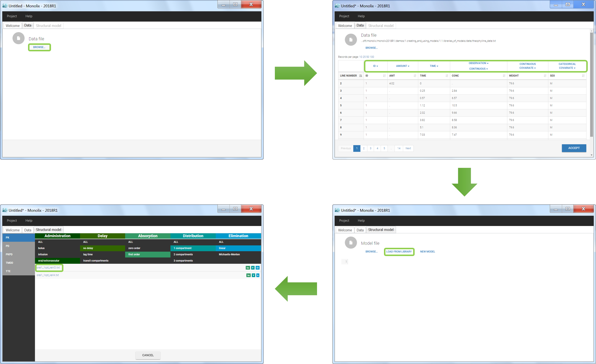
We would like to set up a one compartment PK model with first order absorption and linear elimination for the theophylline data set. We start by creating a new Monolix project. Next, the Data tab, click browse, and select the theophylline data set (which can be downloaded from the data set documentation webpage). In this example, all columns are already automatically tagged, based on the header names. We click ACCEPT and NEXT and arrive on the Structural model tab, click on LOAD FROM LIBRARY to choose a model from the Monolix libraries. The menu at the top allow to filter the list of models: after selecting an oral/extravascular administration, no delay, first-order absorption, one compartment and a linear elimination, two models remain in the list (ka,V,Cl) and (ka,V,k). Click on the oral1_1cpt_kaVCl.txt file to select it.

After this step, the GUI moves to the Initial Estimates tab, but it is possible to go back to the Structural model tab to see the content of the file:

[LONGITUDINAL]
input = {ka, V, Cl}

EQUATION:
Cc = pkmodel(ka, V, Cl)

OUTPUT:
output = Cc

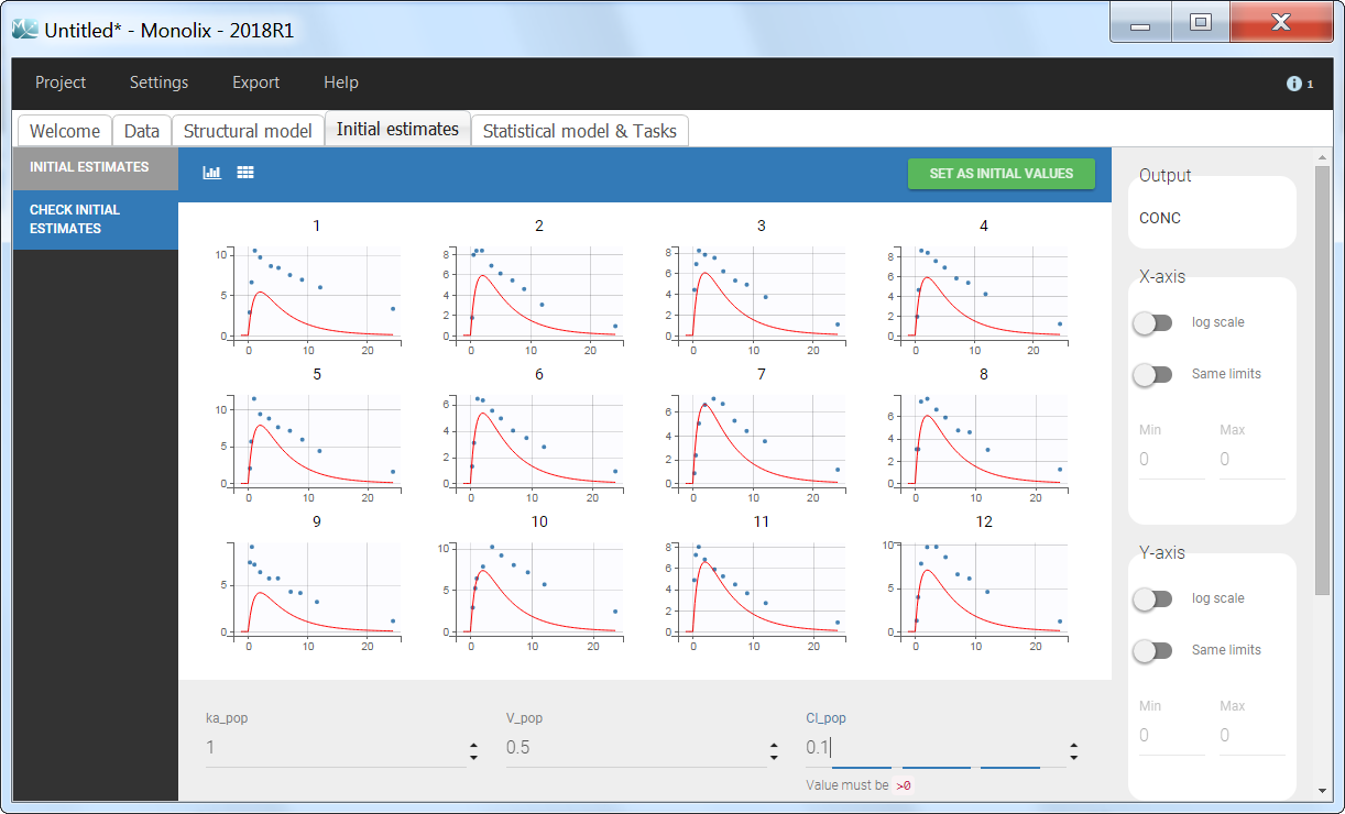
Back to the Initial Estimates tab, the initial values of the population parameters can be adjusted by comparing the model prediction using the chosen population parameters and the individual data. Click on SET AS INITIAL VALUES when you are done.

In the next tab, the Statistical model & Tasks tab, we propose by default:

• A combined error observation model
• Lognormal distributions for all parameters (ka, V and Cl)

At this stage, the monolix project should be saved. This creates a human readable text file with extension .mlxtran, which contains all the information defined via the GUI. In particular, the name of the model appears in the section [LONGITUDINAL] of the saved project file:

<MODEL>
[INDIVIDUAL]
input = {ka_pop, omega_ka, V_pop, omega_V, Cl_pop, omega_Cl}

DEFINITION:
ka = {distribution=lognormal, typical=ka_pop, sd=omega_ka}
V = {distribution=lognormal, typical=V_pop, sd=omega_V}
Cl = {distribution=lognormal, typical=Cl_pop, sd=omega_Cl}

[LONGITUDINAL]
input = {a, b}
file = 'lib:oral1_1cpt_kaVCl.txt'

DEFINITION:
CONC = {distribution=normal, prediction=Cc, errorModel=combined1(a,b)}