Missing observations can cause a bias in the VPC and hamper its diagnosis value. This mini case-study shows why missing censored data or censored data replaced by the LOQ can cause a bias in the VPC, and how Monolix handles censored data to prevent this bias. It also explains the bias resulting from non-random dropout, and how this can be corrected with Simulx.
Censored data and VPC
This section explains the different cases that can occur when some data are censored. If the censored data are marked in the dataset, they are handled by Monolix in a way that prevents bias in the diagnostic plots such as the VPC. The bias remains however if the censored data are missing.
Censored data missing from the dataset
The figures below show what happens if censored data are missing from the dataset. The figures on the left and middle focus on two individuals in a PK dataset, with their observed concentrations (on the left) or predicted concentrations (in the middle) over time as blue dots, and with similar measurement times. We assume that a good model has been estimated on this data. Three simulated replicates are represented on the same plot in the middle, although percentiles are calculated on each replicate separately in order to generate the prediction intervals on the VPC.
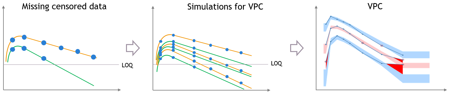
In case of missing censored data, the empirical percentiles represented by the blue lines on the VPC do not decrease much at high times, because only the individuals with high enough observations (like the orange individual, and not like the green individual) contribute to the percentiles.
The simulations for the VPC follow the same measurement times as the initial dataset, however if the variability is unexplained the predictions for all the individuals have the same prediction distributions, so the number of predicted observations that contribute to the prediction intervals are the same for each percentile. This results in a discrepancy between observed and simulated data, that can be seen in red.
Explained inter-individual variability
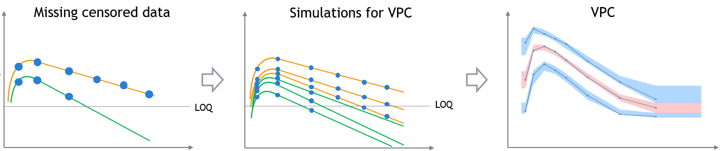
This bias is reduced if most of the variability in the predictions is explained by some covariate effects in the model. In that case the variability of the predicted concentrations at high times will match the variability in the measurement times, and the discrepancy is reduced and can diseappear. The diagnosis value of the VPC is improved, although the shape of the percentiles in the VPC is still affected by missing observations.
Censored data in dataset and “Use censored data” is OFF
If there is censored data in the dataset and the toggle “use censored data” in VPC plot display settings is off, the VPC is simulated for all times including censored times, and all values below the maximum LLOQ value and above the minimum ULOQ in dataset are dropped to calculate the percentiles.
The empirical percentiles are calculated using the non-censored times only.
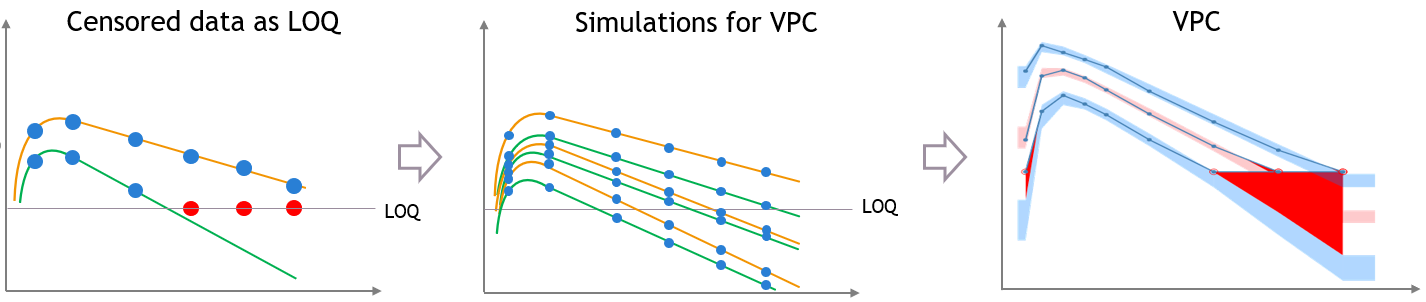
“Use censored data” is ON and LOQ is used for calculations
In this case, the VPC is simulated for all times including censored times, and all simulated values are used to calculate the simulated percentiles.
For the empirical percentiles, the LOQ value in the dataset is used to replace the censored observations in the percentile calculation.
A strong bias appears in the VPC. The bias affects the empirical percentiles, as seen below, because the censored observations should actually be lower than the LOQ.
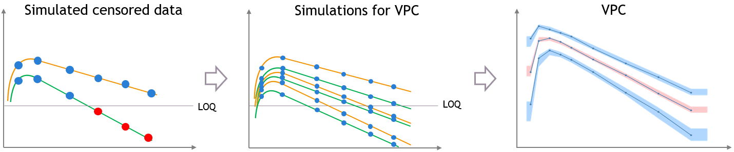
“Use censored data” is ON and simulated observations are used for calculations
In this case, the VPC is simulated for all times including censored times, and all simulated values are used to calculate the simulated percentiles.
For the empirical percentiles, the bias shown above is prevented by replacing the censored observations in the diagnostic plots by samples from the conditional distribution \(p(y^{BLQ} | y^{non BLQ}, \hat{\psi}, \hat{\theta})\), where \(\hat{\theta}\) and \(\hat{\psi}\) are the estimated population and individual parameters.
This corrects the shape of the empirical percentiles in the VPC, as seen on the figure below. More information on handling censored data in Monolix is available here.
Dropout and VPC
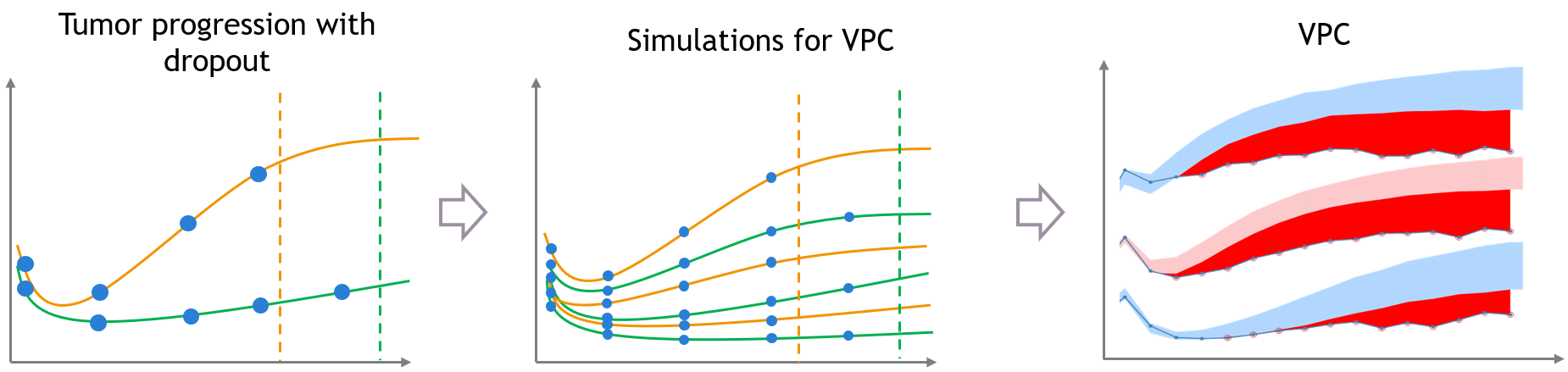
The same kind of bias can also occur when the dataset is affected by non-random dropout events. In this section we take an example of tumor growth data. We assume that the data have been fitted with a good model, and is affected by non-random dropout, because individuals with a high tumor size quit the study or die. This means that no more observation for the tumor size is available after the time of dropout, represented with the dashed vertical lines.
A bias appears in the VPC, caused by the missing censored observations. This is because there are more missing observations in the dataset for high tumor sizes, which is not the case in simulated predictions from the model, unless the inter-individual variability is well explained by some covariate effects.
Correcting the bias from dropout
Correcting this bias requires to provide additional measurement times after the dropouts, which cannot be done automatically in Monolix without making strong assumptions on the design of the dataset. However, it can be attempted with simulations in Simulx, with additional measurement times chosen by the user in adequation with the dataset, and some post-processing in R.
The correction also requires to model the dropout with a time-to-event model, that should depend on the tumour size. After estimating the joint tumor growth and time-to-event model in Monolix, it becomes possible to predict the time of dropout for each individual. The predictions for dropout times we will use for post-processing in R.
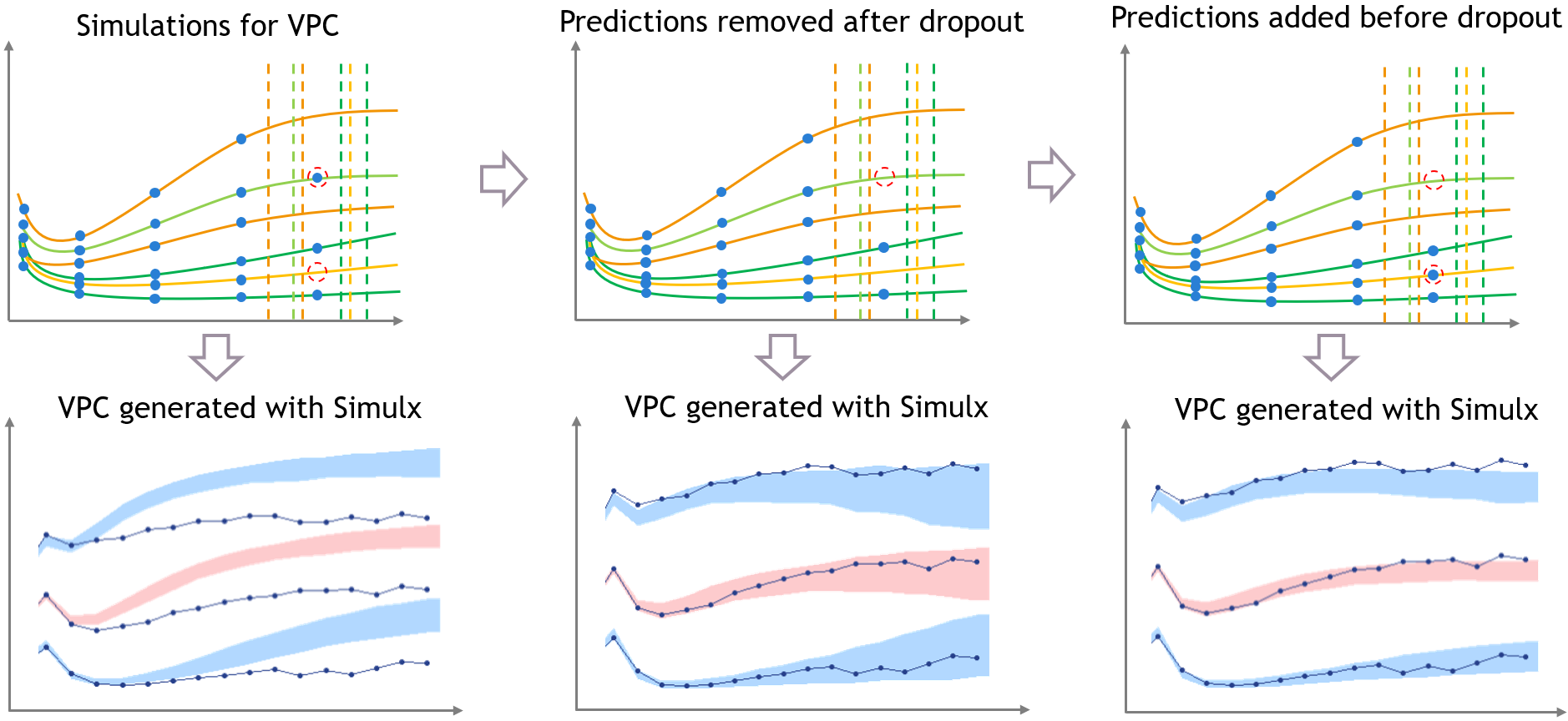
The figure below shows the main steps for correcting the bias from dropout in a VPC. The VPC (on the bottom of the figure) can be regenerated with new simulations in Simulx (shown on the top of the figure) and with some plotting functions of ggplot to display the empirical percentiles and prediction intervals. Two simulations that can be corrected are colored in light orange and in light green.
First, the light green simulation comes from an individual that had a late dropout in the initial dataset, so it has late prediction times. However, in this case the predicted tumor size if high, and the predicted dropout, visible in light green dashed line, occurs before the last prediction time. If this individual was real, it would not have been possible to measure this observation. (Note that for Monolix or Simulx the dropout is just an event, it cannot have any effect on the predictions of the size model
Second, the light orange simulation comes from the orange individual, so it has missing predictions at high times. However in this case the predicted tumor size is small and the predicted dropout time is quite high, higher than the missing predictions. So if this individual was real, it would have been possible to measure an additional observation here.
- Step 1 (left): the VPC is displayed without post-processing: it has the same bias as in Monolix.
- Step 2 (middle): To get predictions that are more representative of the dataset, the prediction marked in red from the light green simulation is removed before plotting the VPC, along with all the individual predictions that occur after the corresponding predicted dropout. This first correction is seen in the middle and reduces strongly the bias of the VPC.
- Step 3 (right): With Simulx it is possible to change the design structure for the prediction times defined in the outputs of the simulations. The time marked in red for the light orange simulation is added in the output before performing the simulations for the VPC, and the same is done for all individuals that have missing observations in the dataset.
Combining the pre-processing of the outputs before the simulations from Step 3 and the post-processing of the simulations from Step 2 to remove the predictions occurring after a dropout gives a VPC that is not biased by a spurious discrepancy (VPC3). The shape of the percentiles in the VPC is still affected by the dropouts, but the diagnosis value of the VPC is retained.
The difficulty of the approach in Step 3 is to extrapolate the design of the dataset in a way that makes sense. This can not be done in Monolix, but it has to be done in R by the user because it requires to make assumptions on the design, and it might be problematic when the design structure is complex.
For example, in the case of repeated doses, doses that are missing from the dataset because they would occur after a dropout will also have to be included in the new design. Furthermore, the user has to extrapolate the measurement times from the dataset, that are not necessarily the same for all individuals, while keeping the same measurement density for the new observations as for the rest of the observations, to avoid introducing other bias in the VPC.
Example
The example shown on this page along with the R script to correct the VPC can be downloaded here:
This example is based on simulated data from the PDTTE model developed in “Desmée, S, Mentré, F, Veyrat-Follet, C, Sébastien, B, Guedj, J (2017). Using the SAEM algorithm for mechanistic joint models characterizing the relationship between nonlinear PSA kinetics and survival in prostate cancer patients. Biometrics, 73, 1:305-312.” We assume for the sake of the example that the level of PSA is a marker of the tumour size.