Download data set only | Monolix project files | Simulx project files and scripts
⚠️ Under construction ⚠️
This case study presents the modeling of the tobramycin pharmacokinetics, and the determination of a priori dosing regimens in patients with various degrees of renal function impairment. It takes advantage of the integrated use of Monolix for data visualization and parameter estimation and Simulx for simulations and best dosing regimen determination.
The case study is presented in 4 sequential parts, that we recommend to read in order:
- Part 1: Introduction
- Part 2: Exploratory Data Analysis with Monolix
- Part 3: Model development with Monolix
- Part 4: Simulations for individualized dosing with Simulx and Monolix
Part 4: Simulations for individualized dosing with Simulx and Monolix
- A glance at Simulx possibilities
- Safety and efficacy of the usual treatment
- A priori determination of an appropriate dosing regimen for a specific individual
- Using the individuals covariates
- Using the individuals parameters obtained from therapeutic drug monitoring
- A note on individual predictions for individualized dosing
A glance at Simulx possibilities
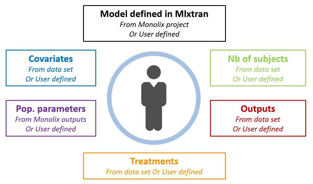
Now that we have a model, we can use it to do simulations. The saved Monolix project can be reused by the R package Simulx for straightforward simulations. All project components (structural model, number of subjects, covariates, treatments, estimated parameter values and outputs) can either be reused from the project or data set, or be redefined by the user.
 After having open R, loaded the mlxR library (containing simulx) via
 library(mlxR) and set the working space, we are ready to start. For instance, to simulate the project without any change, just type:
res1 <- simulx(project = '../monolixProjects/project_07.mlxtran')
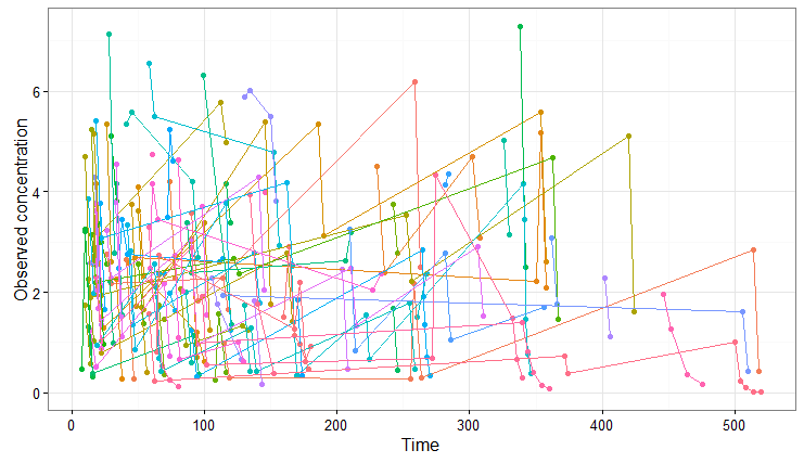
With this call, simulx is able to recover all the information defined in the Monolix project. The covariates and estimated population parameters will be used to draw individual parameter values and these values are then used to do simulations using the same treatments and measurement times as in the original data set.
The results can be plotted with:
print(ggplotmlx(data=res1$y) +
 geom_point(aes(x=time, y=y, colour=id)) +
 geom_line(aes(x=time, y=y, colour=id)) +
 scale_x_continuous("Time") + scale_y_continuous("Observed concentration") +
 theme(legend.position="none"))
We obtain the following spaghetti plot, which is similar but different compared to the original data set:
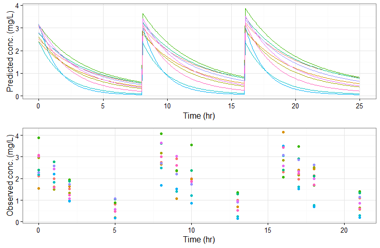
As a second example, we can change the administration schedule to three doses of 80 mg at 0, 8 and 16 hr for all individuals, simulate only 10 individuals (resampled from the data set with their covariates), change the V_pop parameter to a higher value (while keeping the value estimated by Monolix for the other population parameters) and set denser measurement times. Only a few lines are necessary to define the simulations to run:
#====== define project file
project.file <- '../monolixProjects/project_07.mlxtran'

#====== define administration schedule
adm <- list(time=c(0,8,16), amount=80)

#====== define number of individuals
N <- 10

#====== define outputs: both 'y' (with residual error noise) and 'Cc' (predicted concentration)
outy <- list(name = 'y', time = c(0,1,2,5,8,9,10,13,16,17,18,21))
outCc <- list(name = 'Cc', time = seq(0,25, by=0.1))

#===== change V_pop parameter value (others are taken from the estimates.txt file)
param <- c(V_pop=30)

#===== simulate
res2 <- simulx(project = projectfile,
 output = list(outy, outCc),
 treatment = adm,
 group = list(size=N),
 parameter = param)
The predicted exact concentrations and observed concentrations are the following, for the 10 simulated individuals:
Safety and efficacy with the usual treatment
In the present case, we are interested in optimizing the dosing regimen of Tobramycin. Usually Tobramycin is administrated as an intravenous bolus at 1 to 2 mg/kg every 8h (traditional dosing) or at 7 mg/kg once daily (new once-daily dosing). In this case study, we will start with the traditional dosing every 8h, at a dose of 1mg/kg. Higher clinical efficacy has been associated with peak drug concentration in the range 6-7 mg/L. Thus our efficacy target will be 6-7 mg/L for the Cmax, while the trough concentration must be below 2mg/L to avoid toxicity. What percentage of the population meets the efficacy and safety target, if Tobramycin is administrated according to the usual dosing regimen?
To answer this question, we will simulate the default treatment for the individuals of the data set. In the Monolix project, doses are given in mg. We now would like to work with doses in mg/kg, which makes the code slightly more complex than the two examples above, as we need to adapt the dose of each individual depending on its weight. We will read the weight information from the data set using the readDatamlx function and use it to define the administration in a data frame listing the times and amounts for each individual. To simulate the steady-state peak and trough concentration for 1000 individuals, resampled from the data set, receiving 1 mg/kg every 8 hours, we write:
project.file <- '../monolixProjects/project_07.mlxtran'
N <- 1000

# output definition: look at 2 cycles after 35 cycles (to be in steady-state)
outCc <- list(name = 'Cc', time = seq(279, 295.9, by=0.1))

# defining the repeated administration.
# The amount is calculated based on the weight
d <- readDatamlx(project = project.file)
covariates1 <- d$covariate
dosePerKg <- 1
times <- seq(0,300,by=8)
nbTimes <- length(times)
adm1 <- data.frame(id = rep(1:d$N,each=nbTimes),
 time = rep(times,d$N),
 amount = rep(dosePerKg*covariates1$WT,each=nbTimes))

# simulation of N=1000 individuals
res1 <- simulx(project = project.file,
 output = outCc,
 treatment = adm1,
 parameter = d$covariate,
 group = list(size=N))
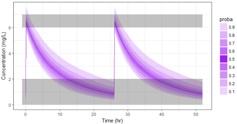
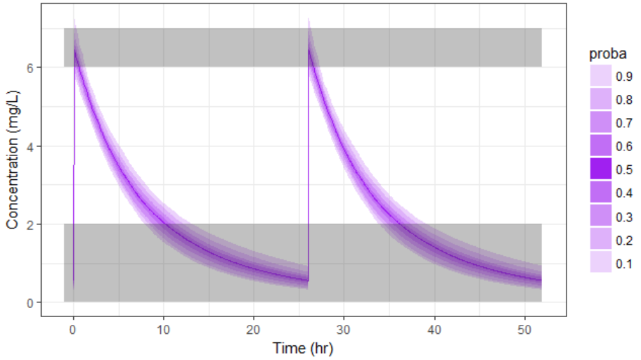
We can then plot the concentration prediction interval with:
pPrct1 <- prctilemlx(res1$Cc, band=list(number=9,level=90)) +
 scale_x_continuous("Time (hr)") +
 scale_y_continuous("Concentration (mg/L)", limits = c(0, 9.5)) +
 ggtitle("with covariates sampled from the data set")
print(pPrct1)
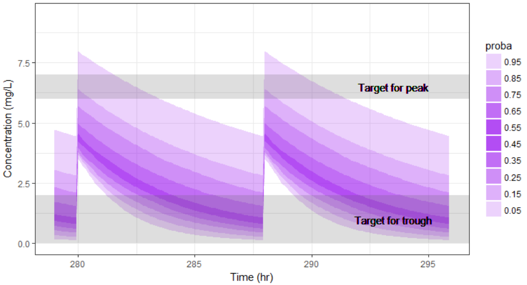
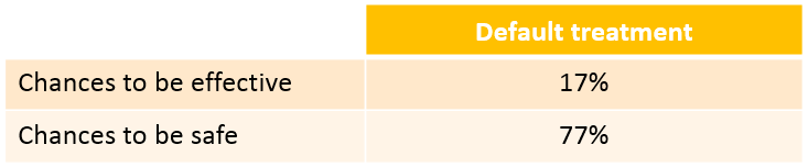
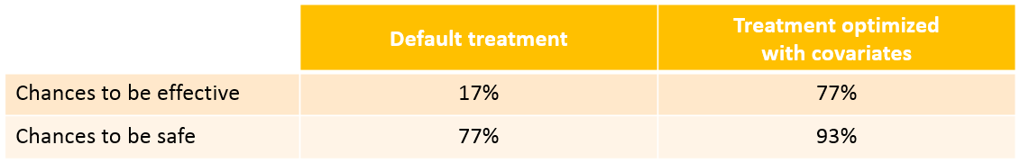
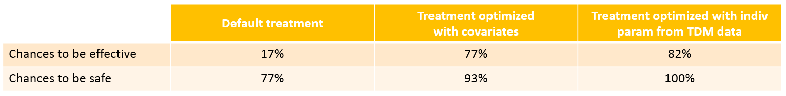
We see that a relatively large fraction of the individuals do not meet the safety criteria, the efficacy criteria or both. Using the simulation results outputted as tables in the res1 object, we can quantify the percentage of people meeting the criteria: with the default treatment, the chances that the treatment is effective are only 17% and the chances that the treatment is safe are 77%.
This calls for an individualization of the dose, to adapt the dosing regimen to the patients characteristics.
A priori determination of an appropriate dosing regimen for a specific individual
The poor performance of the default dosing prone us to adapt the dosing to the patients characteristics. To adapt the dosing, we can either use the patients covariates or try to get even more information of the patient using therapeutic drug monitoring.
Using the individuals covariates
We would like to a priori determine an appropriate dosing regimen for an individual, knowing its covariates values. For instance, we will consider an individual weighting 78 kg, with a creatinine clearance of 30 mL/min, which corresponds to a severe renal impairment. Knowing the covariates, we have an idea of the individual parameters for this individual, but uncertainty remains, which is captured in the random effects. For instance for the elimination rate k we have:
$$k_i=k_{pop}(\frac{CLCR}{67.87})^{\beta_{k,CLCR}}(\frac{WT}{66.47})^{\beta_{k,WT}} e^{\eta_{k,i}}$$
To determine a better dosing regimen than the default dosing for this individual, we will proceed in the following way:
- consider a typical individual with weight 78 kg and creatinine clearance 30 mL/min
- test if the efficacy and safety criteria are met with the default treatment. If not,
- write an optimization algorithm to find a better dosing regimen
- test the chances of the optimized dosing to be safe and efficient by considering the uncertainty of the parameters (i.e putting back the random effects)
We first consider a typical individual with this weight and creatinine clearance, i.e we neglect the random effects. How would the typical treatment perform on this individual? We simulate the patient with the following code. Compared to the previous script, we this time do not take the covariates from the data set but define them ourselves:
# define project file
project.file <- '../monolixProjects/project_2cpt_final.mlxtran'

# an individual with WT=78 and CLCR=30
weight <- 78
clcr <- 30

# define output
outCc <- list(name = 'Cc', time = seq(279, 295.9, by=0.01))

# define covariates
covariates <- data.frame(id = 1, WT = weight, CLCR= clcr)

#disable random effects to simulate typical individual with this WT and CLCR
param=c(omega_k=0,omega_V=0)

# define usual treatment
dosePerKg <- 1
interdoseinterval <- 8
adm <- list(time=seq(0,300,by=interdoseinterval), amount=dosePerKg*weight)

# run simulation of one individual
res <- simulx(project = project.file,
 output = outCc,
 treatment = adm,
 parameter = list(covariates,param))
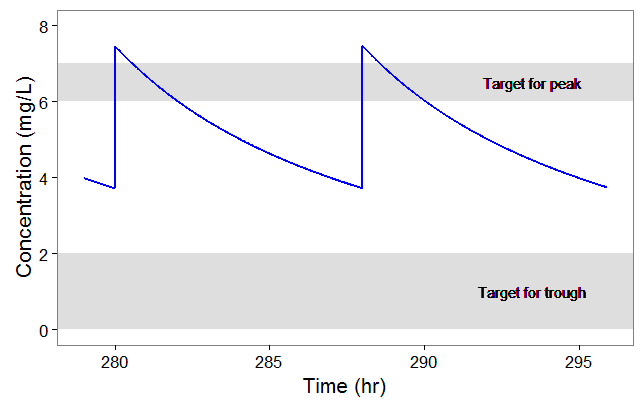
After plotting, we obtain the following figures that shows that for a typical individual with weight 78 kg and creatinine clearance 30 mL/min the trough concentration is too high so the default treatment has a high risk to be toxic.
We thus would like to adapt the dosing regimen for this individual, given its covariates values. We start by implementing a function that returns the peak and trough concentrations at steady-state, for a given dose per kg and a given inter-dose interval:
getMinMax <- function(projectfile,dosePerKg,interdoseinterval, weight, clcr){

 outCc <- list(name = 'Cc', time = seq(35*interdoseinterval-0.05, 35*interdoseinterval+28, by=0.05))
 # define covariates
 covariates <- data.frame(id = 1, WT = weight, CLCR= clcr)

 # define treatment
 adm <- list(time=seq(0,38*interdoseinterval,by=interdoseinterval), amount=dosePerKg*weight)

 #disable random effects
 param=c(omega_k=0, omega_V=0)

 # run simulation of one individual
 N <- 1
 res <- simulx(project = projectfile,
 output = outCc,
 treatment = adm,
 parameter = list(covariates,param))

# set starting time to zero for easier comparison
 Conc <- res$Cc
 Conc$time <- Conc$time - Conc$time[1]

 maxi <- Conc[which(diff(sign(diff(Conc$Cc)))==-2)+1,]
 mini <- Conc[which(diff(sign(diff(Conc$Cc)))==2)+1,]

 result <- list(min=mini$Cc[1], max=maxi$Cc[1])
 return(result)
}
We then implement a simple optimization algorithm: if the peak is too high or too low, the dose is decreased or increased respectively. If the trough is too high, the inter-dose interval is increased. The code reads:
#initial dosing regimen
dosePerKg <- 1
interdoseinterval <- 8
weight <- 78
clcr <- 30
result <- getMinMax(project.file, dosePerKg, interdoseinterval, weight, clcr)

while(result$max < 6.3 | result$max > 6.7 | result$min> 1){
 if (result$max < 6.3 | result$max > 6.7){
 dosePerKg = dosePerKg + 0.2*(6.5-result$max)
 }else if(result$min > 1){
 interdoseinterval = interdoseinterval + 3
 }else{
 paste0("Error")
 }
 result <- getMinMax(project.file, dosePerKg, interdoseinterval, weight, clcr)
}
In the video below, one can visualize how the dose and the inter-dose interval evolve from the initial default treatment to a treatment achieving both efficacy and safety. For this individual, we propose 1.55 mg/kg administrated every 26 hr.
The proposed inter-dose interval may not be feasible in clinical practice. We can either take another close value, for instance 24h or modify the optimization algorithm to take into account the clinical practice constraints. In addition, instead of using a hand-made optimization algorithm, it is also possible to use more advanced algorithms implemented in separate R packages.
For the optimization above, we have considered a typical individual among the population of people with WT=78 and CLCR=30. We will now verify the chances of the optimized treatment to be safe and efficient, taking into account the uncertainty of the individual parameters for this individual, via the random effects.
The code is as follows. The only difference is that we do not disable the random effects anymore and simulate the individual 100 times to get a prediction distribution.
#output
outCc <- list(name = 'Cc', time = seq(35*interdoseinterval-0.05, 37*interdoseinterval-0.05, by=0.05))

# to get
N <- 100

# define covariates
 covariates <- data.frame(id = 1, WT = weight, CLCR= clcr)

# define optimized treatment
adm <- list(time=seq(0,38*interdoseinterval,by=interdoseinterval), amount=dosePerKg*weight)

# run simulation of one individual, parameter k is drawn
#from its distribution, taking into account the covariates
res <- simulx(project = project.file,
 output = outCc,
 treatment = adm,
 parameter = covariates)
With the optimized treatment for this individual, there are 93% chances that the treatment is safe and 77% chances that it is effective. This is an improvement compared to the default treatment:
Yet if one would have a better estimate of the parameters for this individual instead of only its covariates information, one would be able to even better calibrate the dosing schedule. This is possible using therapeutic drug monitoring.
Using the individuals parameters, obtained from therapeutic drug monitoring (TDM)
After the first drug injection, it may be useful to monitor the drug concentration in order to adapt the subsequent doses. The goal is to use the measured concentrations to determine the parameters of this individual and use these estimated parameters to simulate the expected concentration range after several doses and adapt the dosing accordingly.
Let’s assume that for our individual (weight=78 kg, creatinine clearance=30 mL/min), we have started with the a priori proposed dose 93.6 mg, and have measured the concentration at a few time points after the first dose:
ID   TIME  DOSE     Y  WT  CLCR
1     0    93.6     .  78   30
1     1    .     3.59  78   30
1     3    .     2.75  78   30
1     5    .     2.07  78   30
1     8    .     1.11  78   30
We can use Monolix to estimate the individual parameters of this individual, fixing the population parameters to those estimated previously. In the monolix project below, the model is exactly the same as the final model determined using the clinical data set, the population parameters have been fixed to the estimated values and the data set has been replaced by the one above, recording the TDM measurements for this individual:
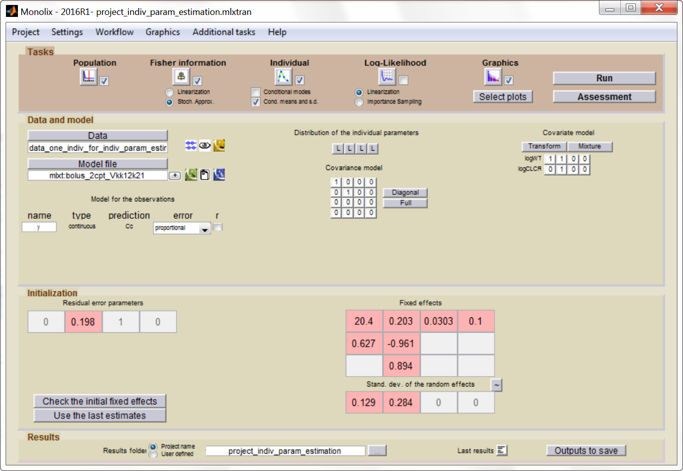
After having run the estimation of the population parameters (which just prints the parameters to a file, as all population parameters are fixed), we can estimate the mean, mode and std of the conditional distribution ")
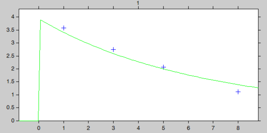
The “IndividualFits” graphic shows the prediction using the estimated conditional mean and the drug monitoring data:
Click here to download the Monolix project to estimate the individual parameters.
We now would like to use the estimated individual parameters to adapt the treatment. In Simulx, it is not possible to directly set the value of the parameters at the individual level when using a project file as input. We will instead work with a model file as input, containing the structural model. In a very similar manner as previously, we define a getMinMax function (below) and an optimization loop. The parameters V, k, k12 and k21 are set to the mean of the conditional distribution calculated with Monolix.
getMinMax_withModel <- function(modelfile, dosePerKg,interdoseinterval, reference, weight,clcr){

 outCc <- list(name = 'Cc', time = seq(35*interdoseinterval-0.05, 35*interdoseinterval+28, by=0.05))

 # parameter values fixed
 parameters <- data.frame(id = 1,
 V = 23.8,
 k = 0.112,
 k12 = 0.0303,
 k21 = 0.1)

 # define treatment
 adm <- list(time=seq(0,38*interdoseinterval,by=interdoseinterval), amount=dosePerKg*weight)

 # run simulation of this individual
 res <- simulx(model = modelfile,
 output = outCc,
 treatment = adm,
 parameter = parameters)

 Conc <- res$Cc
 Conc$time <- Conc$time - Conc$time[1]

 maxi <- Conc[which(diff(sign(diff(Conc$Cc)))==-2)+1,]
 mini <- Conc[which(diff(sign(diff(Conc$Cc)))==2)+1,]

 result <- list(min=mini$Cc[1], max=maxi$Cc[1], ref=reference)
 return(result)
}
The optimization leads to the following schedule: 1.80 mg/kg every 26 hr.
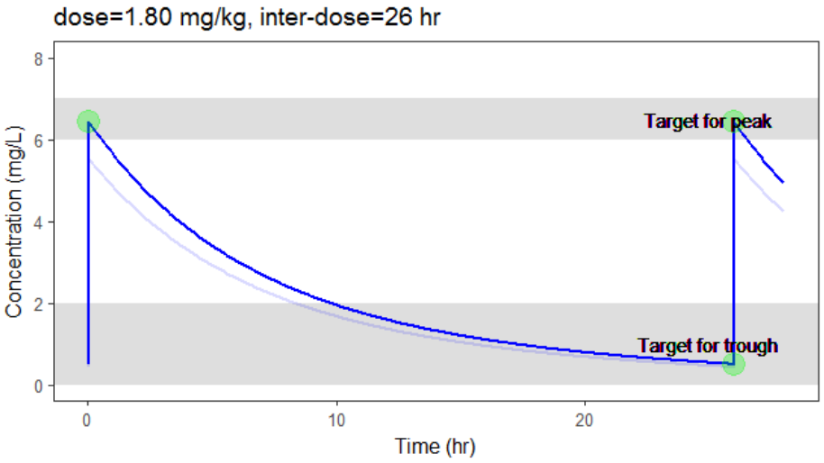
Due to the uncertainty in the individual parameters for this individual, there is also an uncertainty on the simulated concentration.
To verify the chances of the optimized treatment to be safe and efficient, we would like to take into account the distribution of the individual parameter instead of only the mean. The distribution of the individual parameters is a joint distribution (without analytical formula), that can for instance be estimated via a Monte-Carlo procedure. As Monolix does not permit to directly output the result of the Monte-Carlo procedure, we use the following trick: we can set the number of chains (i.e the number of times the data set is replicated) to a high number, which permit to simulate several times the same individual. This is done in Settings > Pop. parameters > nb chains. Then, in the covariates graphic, with the “simulated parameter” option, Monolix draws one parameter value from the conditional distribution per individual (so 1000 if one has used 1000 chains for instance). These values can be outputted to a file by going to Graphics > Export graphics data.
Click here to download the associated Monolix project
The values in the outputted file are thus draws from the joint conditional distribution and represent the uncertainty of the individual parameters. We can use them to simulate the prediction interval for the concentration.
N <- 1000

# load individual parameter values from covariates graphic
file.indiv.param <- '../monolixProjects/project_indiv_param_estimation_1000chains
                     /GraphicsData/Covariates/Covariates_Simul.txt'
data <- read.table(file.indiv.param, header = TRUE, stringsAsFactors = FALSE)

V_ind <- exp(data[data$Cov_WT==78,'Param_log.V.'])
k_ind <- exp(data[data$Cov_WT==78,'Param_log.k.'])

# parameter values
parameters <- data.frame(id  = (1:N),
                         V  = V_ind[1:N],
                         k  = k_ind[1:N],
                         k12 = 0.0303,
                         k21 = 0.1)

# run simulation of N individual, parameter k is drawn from its distribution
outparam <- c("V","k","k12","k21")
res2 <- simulx(model = structuralModelFile,
 output = list(outCc,outparam),
 treatment = adm,
 parameter = parameters)

# calculate the percentiles and plot
pPrct2 <- prctilemlx(res2$Cc, band=list(number=9,level=90)) +
 scale_x_continuous("Time (hr)") +
 scale_y_continuous("Concentration (mg/L)") + ylim(c(0,7.5))

print(pPrct2)
With the newly optimized treatment, there are 82% chances that the treatment is effective and 100% chances that it is safe, which is an improvement compared to the treatment proposed using the covariates only.
A note on individual predictions for individualized dosing
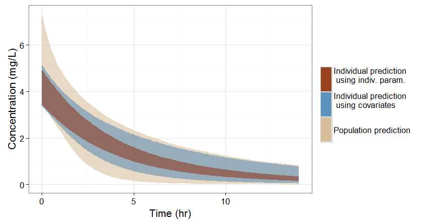
In the previous sections, we have seen three ways of predicting the concentration time course of an individual:
- If no covariate information is available for this individual, we only know that the concentration time course for the individual will be within the prediction interval of the entire population, which is pretty large (tan color in the figure below).
- If the covariates of this individual are available, we can use them to get a reduced distribution of the parameters k and V for this individual. The associated concentration prediction (bleu color in the figure) is narrower compared to the first case.
- If in addition to the covariates, a few measures can be made (drug monitoring), the conditional distribution of parameters k and V (given theses measures and the previously estimated population parameters) can be obtained. This leads to an even more narrow concentration prediction interval (brown in the figure).
Note that for this figure we have used a more typical individual without renal impairment (CLCR=80 mL/min).
Conclusion
This example shows how a personalized treatment can be proposed using population PK modeling and simulation, and how the MonolixSuite software components facilitate an efficient implementation. The modeling/simulation approach permits to precisely assess the trade-off between the prediction precision and the costs of information acquisition. Covariates are usually relatively cheap to measure but in the present case lead to only a moderate reduction of the prediction interval. On the other hand, therapeutic drug monitoring is more expensive but permits a strong narrowing of the concentration prediction interval, which in turn permits a better determination of an effective and safe dosing regimen.