Download data set only | Monolix project files | Simulx project files and scripts
[project files coming soon]
⚠️ Under construction ⚠️
This case study presents the modeling of the tobramycin pharmacokinetics, and the determination of a priori dosing regimens in patients with various degrees of renal function impairment. It takes advantage of the integrated use of Monolix for data visualization and parameter estimation and Simulx for simulations and best dosing regimen determination. The case study is presented in 4 sequential parts, that we recommend to read in order:- Part 1: Introduction
- Part 2: Exploratory Data Analysis with Monolix
- Part 3: Model development with Monolix
- Part 4: Simulations for individualized dosing with Simulx and Monolix
Part 3: Model development with Monolix
- Set up of a Monolix project: definition of data, structural and statistical model for the initial model
- Running tasks on the initial model
- Estimation of the population parameter
- Estimation of the individual parameters
- Estimation of the standard errors of the parameters, via the Fisher Information Matrix
- Estimation of the log-likelihood
- Generation of the diagnostic plots
- Model assessment using the diagnostic plots
- Covariate search
- Test of a two compartment model
- Identification of the observation error model
- Convergence assessment
- Overview
Set up of a Monolix project: definition of data, structural and statistical model for the initial model
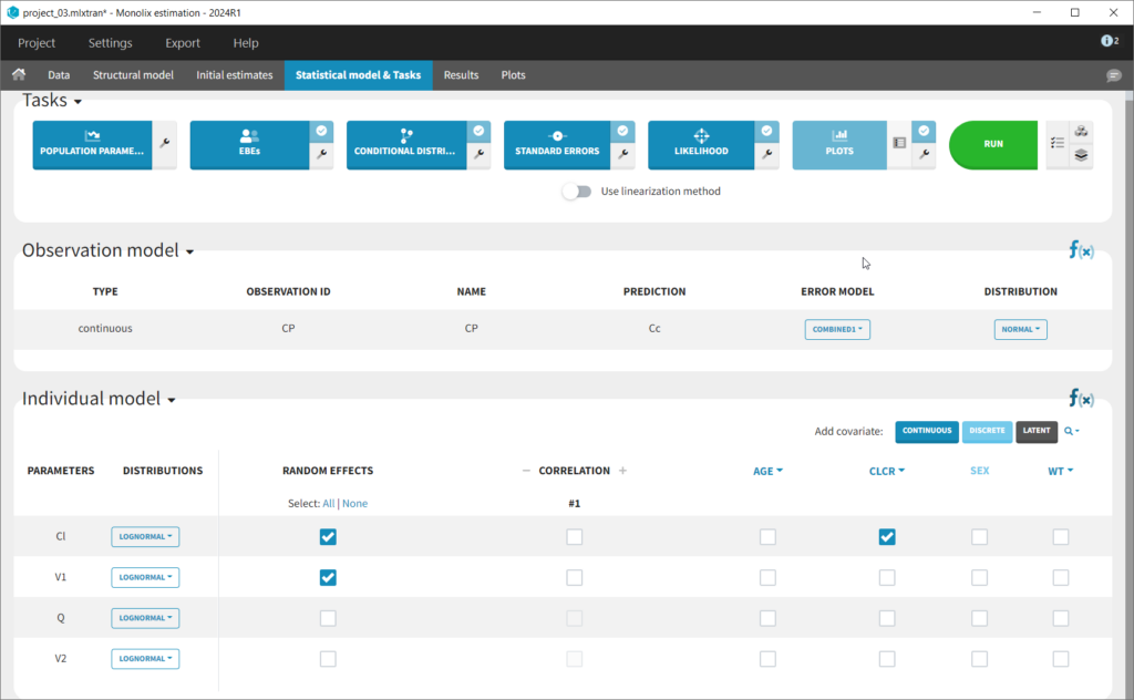
The setup of a Monolix project requires to define the data set, and the model, both the structural part and the statistical part, including the residual error model, the parameter distributions (variance-covariance matrix) and the covariate model. We will setup a first model and improve it step-wise. We first create a new project in Monolix and load the data, assigning the columns as we have done in Datxplore. After having clicked “Next”, the user is prompted to choose a structural model. As a first guess, we try a one-compartment model with bolus administration and linear elimination. This model is available in the Monolix PK library, which is accessed when clicking on “Load from Library > PK”. A (V,Cl) and a (V,k) parameterization are available. We choose the V,k one: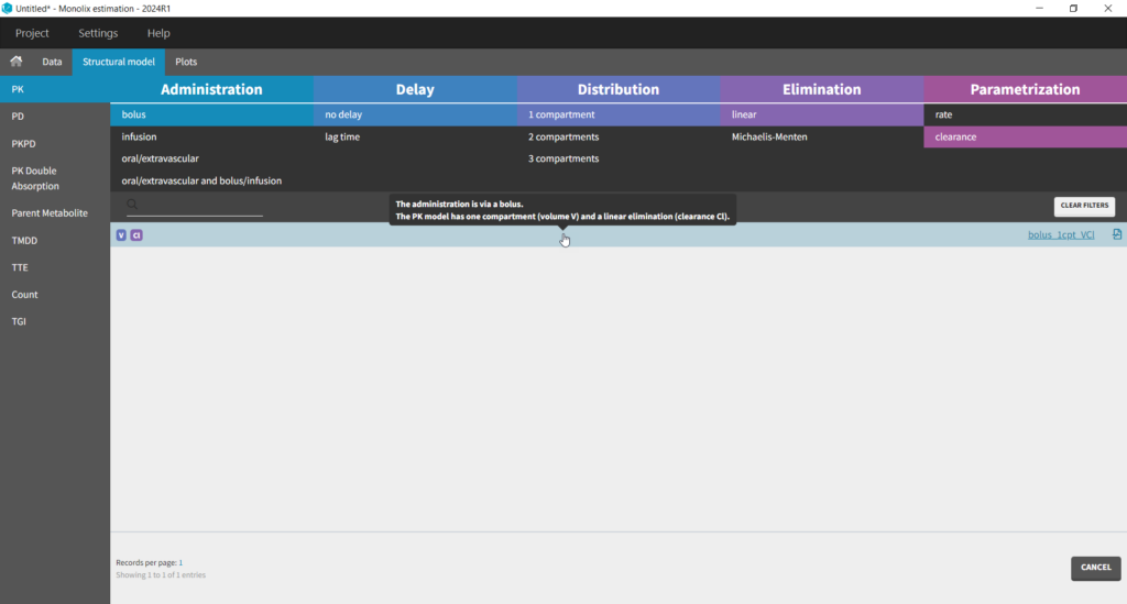
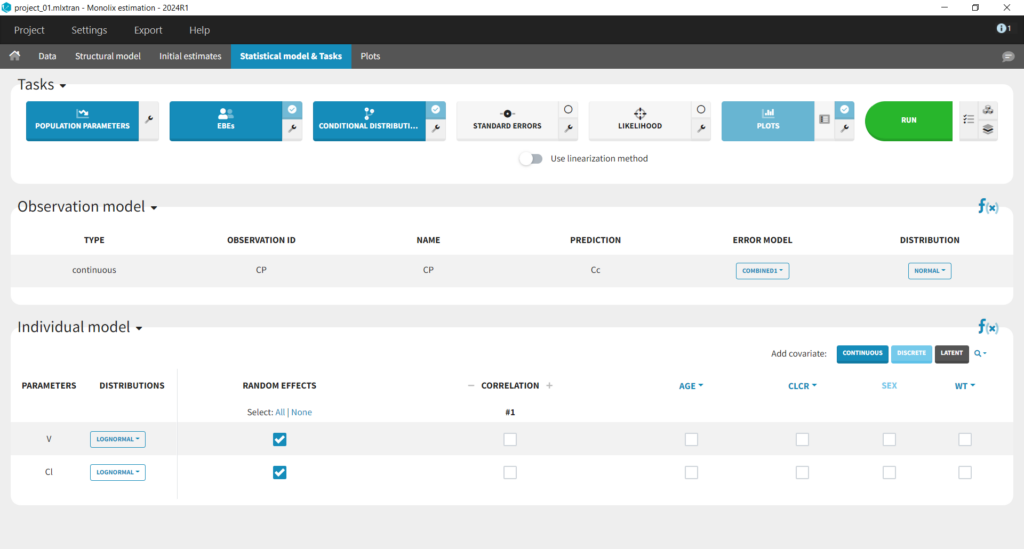
This brings us to the Statistical model & Tasks tab where we can setup the statistical part of the model and run estimation tasks. Under “Observation model,” we define the residual error model. We start with the default combined1 model with an additive and a proportional term, and we will evaluate alternatives later. Under “Individual model,” we define the parameter distributions. We keep the default: log-normal distributions for V and Cl, and no correlations. For now we ignore the covariates.
Running tasks
A single task can be run by clicking on the corresponding button under Tasks. To run several tasks in a row, tick the checkbox in the upper right corner of each task you want to run (it will change from white to blue) and click the green run button. After each task, the estimated values are displayed in the Results tab and output as text files in the result folder with the same name as and next to the Monolix project.Estimation of the population parameters
To run the maximum likelihood estimation of the population parameters, click on the Population Parameters button under Tasks. In the pop-up window, you can follow the progress of the parameter estimates over the iterations of the stochastic approximation expectation-maximization (SAEM) algorithm. This algorithm has been shown to be extremely efficient for a wide variety of even complex models. In a first phase (before the red line), the algorithm converges to the neighborhood of the solution, while in the second phase (after the red line) it converges to the local minimum. By default, automatic termination criteria are used. In the current case, the algorithm shows good convergence: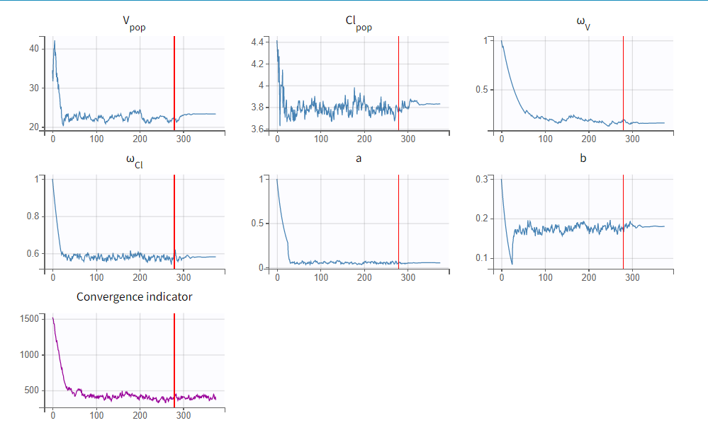
Estimation of the EBEs
The EBEs (empirical Bayes estimates) represent the most probable value of the individual parameters (i.e., the estimated parameter value for each individual). These values are used to calculate the individual predictions that can be compared to the individual data to detect possible mis-specifications of the structural model, for instance. After running this task, the estimated parameter values for each individual is shown in the Results tab and are also available in the results folder > IndividualParameters > estimatedIndividualParameters.txt.Estimation of the conditional distribution
The individual parameters are characterized by a probability distribution that represent the uncertainty of the individual parameter values. This distribution is called the conditional distribution and is specified") . The EBEs are the most probable value of this probability distribution. When an individual has only few data points, the probability distribution may be very large (i.e., large uncertainty). In this case, the EBE values tend to be similar to the population parameter values (shrinkage phenomenon, learn more here) and does not properly represent the individual. The task “Conditional Distribution” samples several (by default 10) possible individual parameter values from the conditional distribution using an MCMC procedure. These values provide a more unbiased representation of the individuals and improve the diagnostic power of the plots.
. The EBEs are the most probable value of this probability distribution. When an individual has only few data points, the probability distribution may be very large (i.e., large uncertainty). In this case, the EBE values tend to be similar to the population parameter values (shrinkage phenomenon, learn more here) and does not properly represent the individual. The task “Conditional Distribution” samples several (by default 10) possible individual parameter values from the conditional distribution using an MCMC procedure. These values provide a more unbiased representation of the individuals and improve the diagnostic power of the plots.
Estimation of the standard errors, via the Fisher Information Matrix
To calculate standard errors of the population parameter estimates, one can calculate the Fisher Information Matrix (FIM). Two options are proposed: via linearization (toggle “Use linearization method” on) or via stochastic approximation (toggle off). The linearization method is faster but the stochastic approximation is usually more precise. As our model runs quickly, we can afford to select the stochastic approximation option and click on the Standard Errors button to calculate the FIM. After the calculation, the standard errors are added to the population parameter table: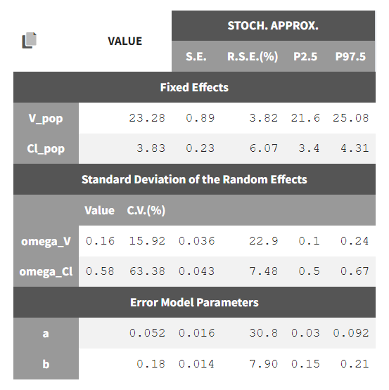
Estimation of the log-likelihood
For the comparison of this model to more complex models later on, we can estimate the log-likelihood, either via linearization (faster, toggle “use linearization method” on) or via importance sampling (more precise, toggle off). Clicking on the Likelihood button under Tasks (with “use linearization method” unchecked), we obtain a -2*log-likelihood of 668, shown in the Results tab under Likelihood, together with the AIC and BIC values. By default, the Standard Errors and Likelihood tasks are not enabled to run automatically. We can click the checkbox to the right of each button to run them automatically when we click the Run button in the future.Generation of the diagnostic plots
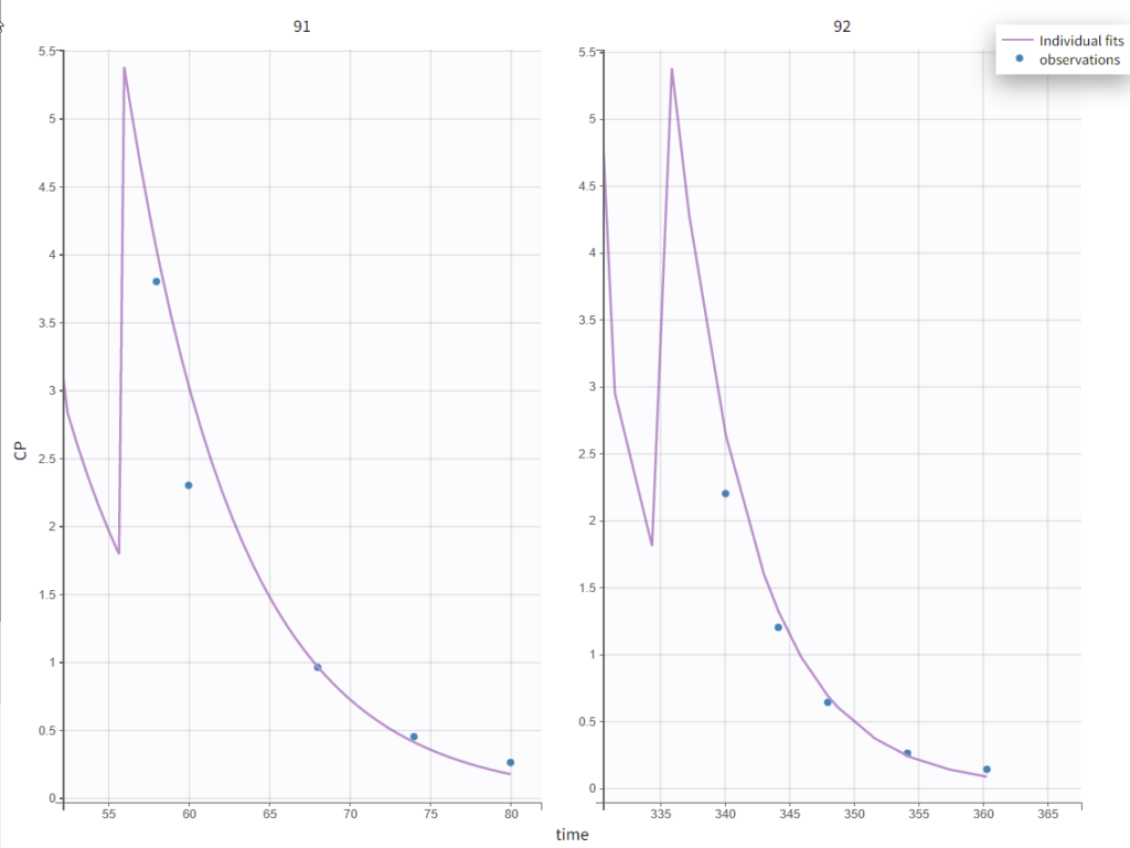
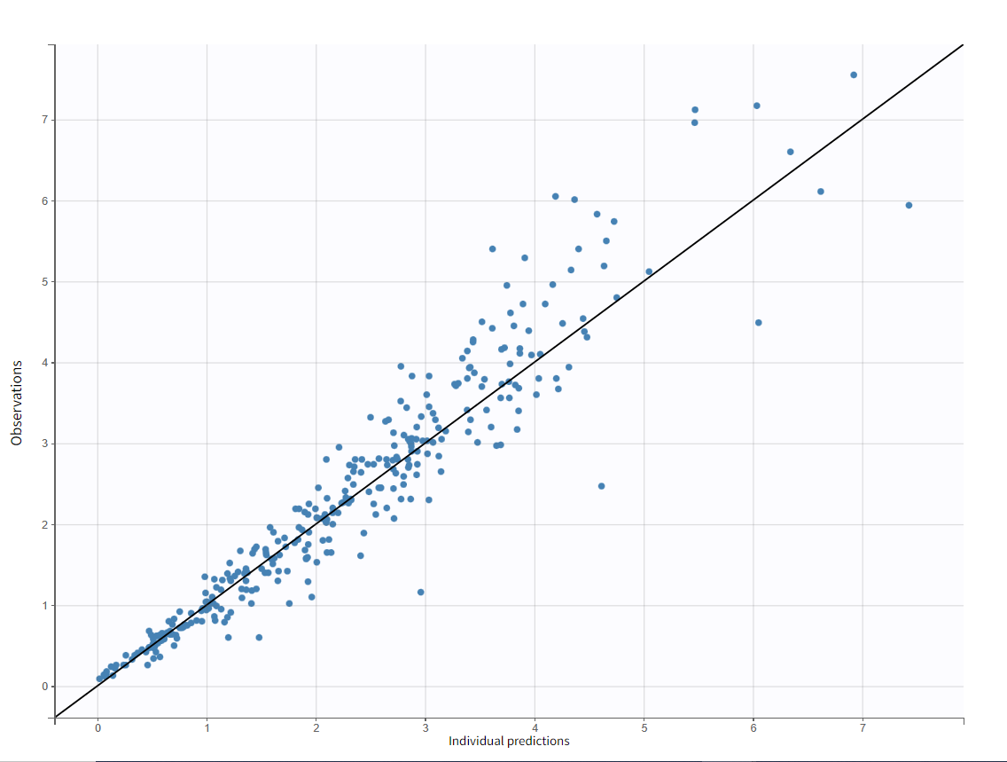
To assess the quality of the model, we finally can generate standard plots. Clicking on the icon next to the Plots button under Tasks, one can see the list of possible figures. Clicking on the Plots button generates the figures.Model assessment using the diagnostic plots
In the “Individual fits” plot, you can choose which individual(s) and how many you would like to display using the buttons in the upper left above the plots: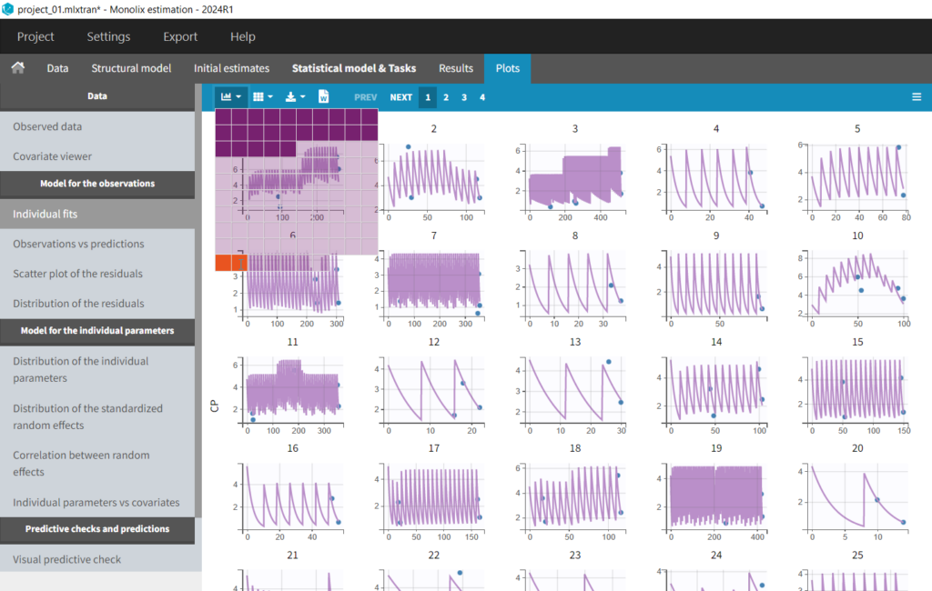
 to obtain an unbiased estimator of
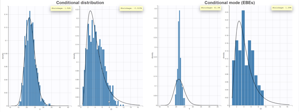
 ") . This allows better detection of parameter distribution mis-specifications. With the “conditional mean” or “conditional mode (EBEs)” options, the shrinkage (specifically the
. This allows better detection of parameter distribution mis-specifications. With the “conditional mean” or “conditional mode (EBEs)” options, the shrinkage (specifically the  -shrinkage, based on the among-individual variation in the model) can be seen (click on “Information” in the General section to display it). The large shrinkage for V means that the data does not allow us to correctly estimate the individual volumes (right side of plot below). Note that the shrinkage is calculated differently in Nonmem and Monolix, see here for more details.
Test of a two-compartment model
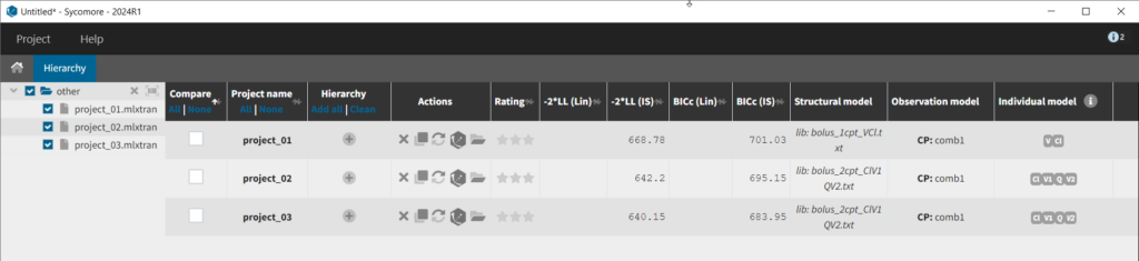
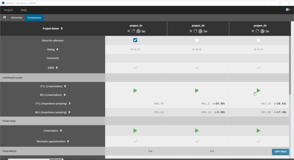
We thus change the structural model to the bolus_2cpt_ClV1QV2 model from the library. We save as project_02 and run the model. Quickly looking at the diagnostic plots, we don’t see any major changes and see that we still have issues fitting the peak in the visual predictive check. However, the -2*LL has dropped to 642. As our data is sparse, we will also try removing the variability on Q and V2, by unselecting the random effects. In this case, all subjects will have the same parameter value for Q and V2 (no inter-individual variability). We save as project_03 and run the model.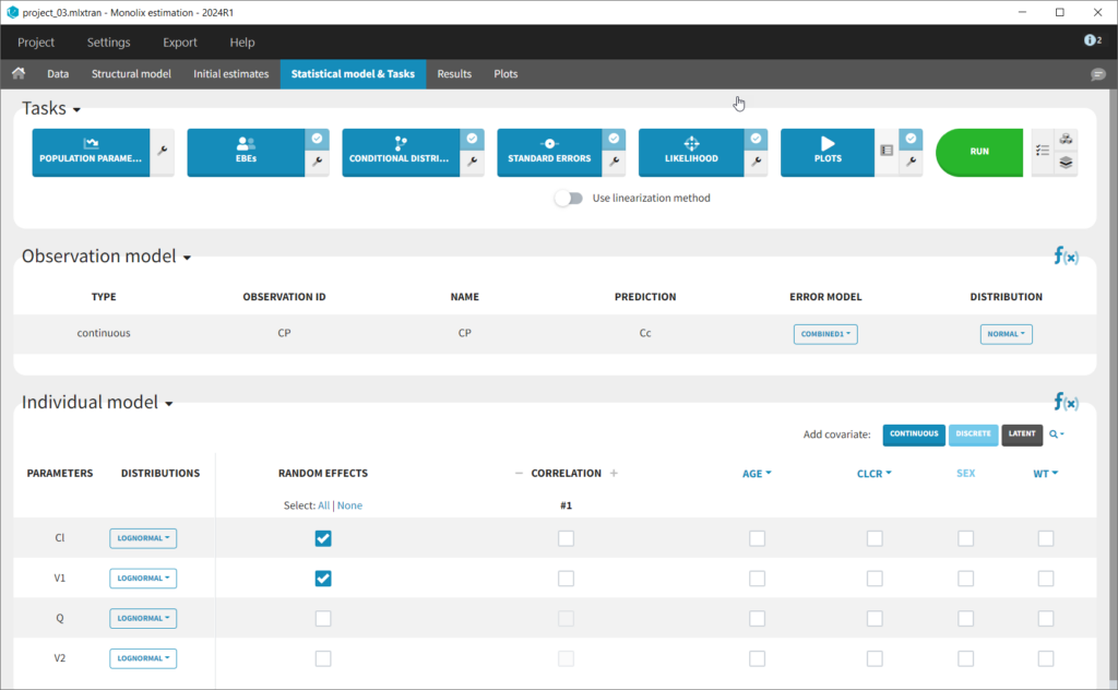
Adding covariates to the model
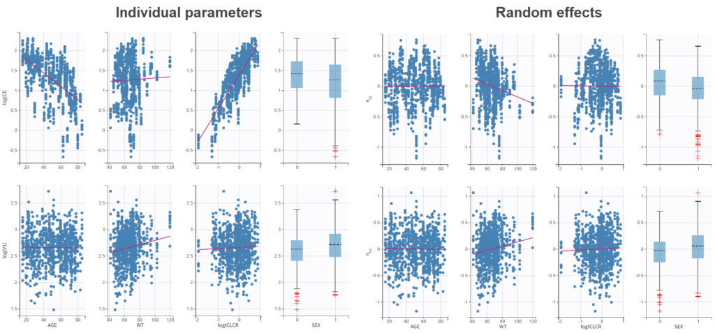
To get an idea of the potential influence of different covariates, we can look at the “Individual parameters vs covariates” plot, where the transformed parameters (log(V) and log(k) as we have chosen log-normal distributions) are plotted against the covariate values. Notice that we use the option “conditional distribution”. This means that instead of using the mode or mean from the post-hoc estimation of each individual parameter, we are sampling from its distribution. This is critical because it is known that the plots using the mode or mean of the post-hoc distribution often show non-existing correlations (see Lavielle, M. & Ribba, B. Pharm Res (2016)).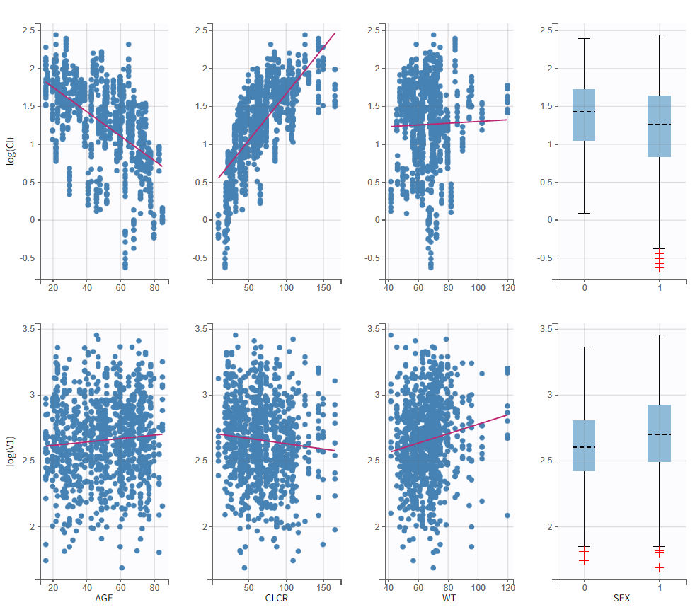
log(Cl)=log(Cl_pop) + beta_Cl_CLCR*CLCR + eta_Cl. So the covariate is added linearly to the transformed parameter. Rewritten, this corresponds to an exponential relationship between the clearance Cl and the covariate CLCR:
$$Cl_i = Cl_{pop} e^{\beta_{Cl,CLCR}\times CLCR_i} e^{\eta_i}$$
with  sampled from a normal distribution of mean 0 and standard deviation
  .
In the “Individual parameters vs covariates” plot, the increase of log(Cl) with CLCR is clearly not linear. So we would like to implement a power law relationship instead:
$$Cl_i = Cl_{pop} \left(\frac{CLCR_i}{65}\right)^{\beta_{Cl,CLCR}} e^{\eta_i}$$
which in the log-transformed space would be written:
.
In the “Individual parameters vs covariates” plot, the increase of log(Cl) with CLCR is clearly not linear. So we would like to implement a power law relationship instead:
$$Cl_i = Cl_{pop} \left(\frac{CLCR_i}{65}\right)^{\beta_{Cl,CLCR}} e^{\eta_i}$$
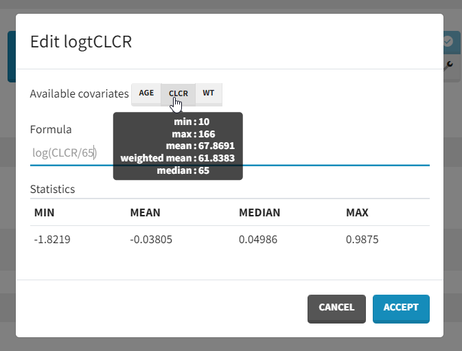
which in the log-transformed space would be written: log(Cl)=log(Cl_pop) + beta_Cl_CLCR*log(CLCR/65) + eta_Cl. Thus, instead of adding CLCR linearly in the equation, we need to add log(CRCL/65).
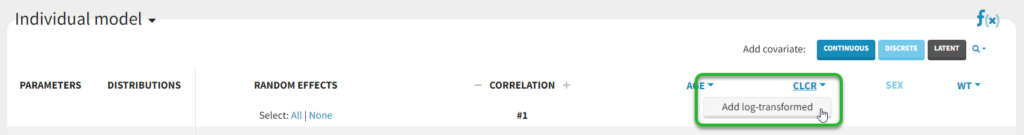
We will create a new covariate logtCLCR = log(CLCR/65). Clicking on the triangle left of CLCR, then “Add log-transformed” creates a new covariate called logtCLCR.
TVCL = THETA(1)*((CLCR/65)**THETA(2))
CL = TVCL * EXP(ETA(1))
with
THETA(1)=Cl_pop, THETA(2)=beta and std(ETA(1))= omega_Cl.
In Monolix, we think in terms of transformed variables:
$$\log(Cl_i) = \log(Cl_{pop})+\beta \times \log(CLCR_i/65) + \eta_i$$
but the two models (in Nonmem and Monolix) are the same, corresponding to:
$$Cl_i = Cl_{pop} \left(\frac{CLCR}{65}\right)^{\beta_{Cl,CLCR}} e^{\eta_i}$$ with sampled from a normal distribution of mean 0 and standard deviation .
We now save the project as project_04, to avoid overwriting the results of the previous run. We then select all estimation tasks and click on Run to launch the sequence of tasks (Population Parameters, EBEs, Conditional Distribution, Standard Errors, Likelihood, and Plots).
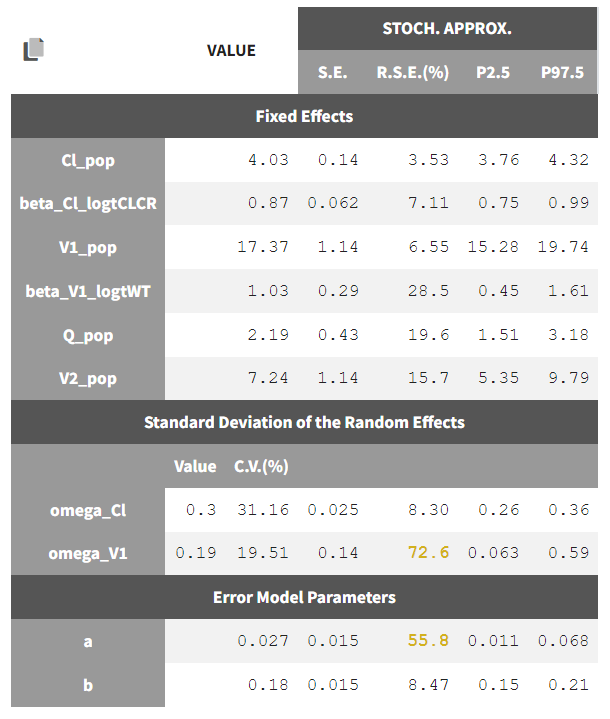
In the Results tab, loking at the population parameters, the effect on CLCR on k is fairly large: for an individual with CLCR=40 mL/min (moderate renal impairment) Cl = 2.6 L/hr, while for an individual with CLCR=100 mL/min (normal renal clearance) Cl = 5.7 L/hr. In addition, the standard deviation of Cl omega_Cl has decreased from 0.56 to 0.31, as part of the inter-individual variability in Cl in now explained by the covariate.
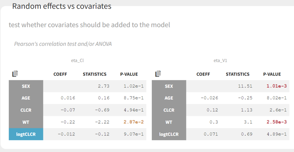
Clicking on Tests on the left shows the results of statistical tests to evaluate adding or removing covariates from the model. under “Individual parameter vs covariates,” we see the results of the correlation test and the Wald test to test whether covariates should be removed from the model. Both tests have a small p-value (< 2.2e-16) for the beta_k_logtCLCR parameter, meaning that we can reject the null hypothesis that this parameter is 0. Under “Random effects vs covariates,” there is a table of tests evaluating adding potential covariates to the model using Pearson’s correlation for continuous covariates and a one-way ANOVA for categorical covariates. Under eta_Cl, logtCLCR is shown in blue, showing it is already accounted for in the model and thus its p-value in non-significant. Small p-values are highlighted in red/orange/yellow and suggest testing the corresponding parameter-covariate relationship if it also makes biological sense. Note that the correlation tests are performed using the samples from the conditional distribution, which avoids bias due to shrinkage. To learn more about how Monolix circumvents shrinkage, see here.The results suggest are three potential covariate relationships to consider: WT on Cl, SEX on V1, and WT on V1. However, because sex and weight are likely correlated (which we can check in the “Covariate viewer” plot), and biologically it would make sense that weight would be correlated with volume, we will first try WT on V1.
Automated covariate search
We could continue testing covariates one by one, by for example testing SEX as a covariate for V1. However, Monolix also provides several methods for automatically searching for covariates. These are accessed by clicking the button “Model Building” (three blocks) to the right of the Run button.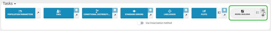
COSSAC
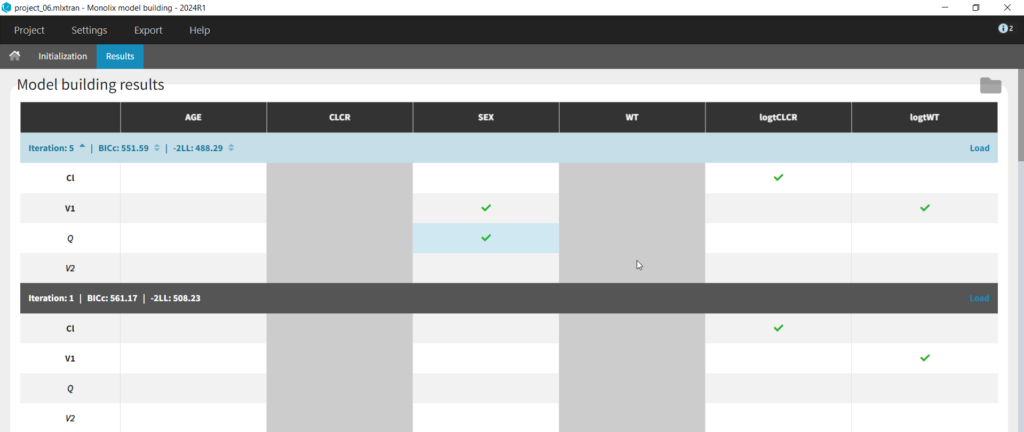
We can first try COSSAC. Because we’ve added log-transformed versions of CLCR and WT, e.g. we want to model a power-law relationship with these covariates, we can disable the non-logged version of these covariates in the covariates dropdown. It’s also possible to force or prohibit specific covariate-parameter relationships by using the lock icons to lock in or lock out specific relationships. Save as project_06, then click run to perform the search.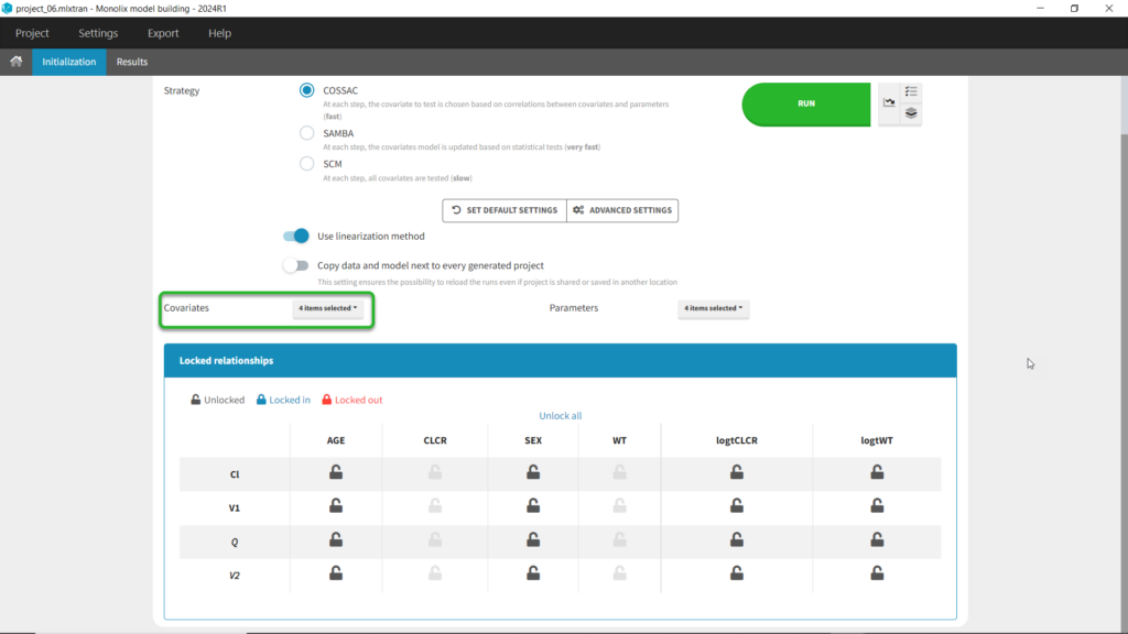
SAMBA
Next we can try SAMBA, which runs very quickly, so can be a good choice for a first approximation for models that take a long time to run. However, one limitation of SAMBA is that parameters without random effects are not included (Q and V2 in our case). Save the project as project_07 and run. Here we see that only two iterations were necessary, and the final model is the same as our final version with logtCLCR on Cl and logtWT on V1. While both iterations contain the same covariates, the likelihoods are slightly different (and an improvement over project_05) due to different parameter estimations influenced by different starting conditions.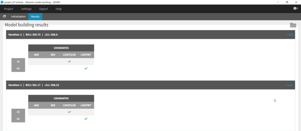
SCM
Finally, we can try the SCM algorithm, the most exhaustive. Select SCM, and after verifying that the appropriate parameters and covariates are selected, save as project_08 and run (be aware this can take some time, ~15-30 min). In our case, the more exhaustive step-wise search performed by SCM took 42 iterations and resulted in the same model selected by COSSAC, that with logtCLCR on Cl,d logtWT on V1, and SEX on both V1 and Q.Identification of the observation error model
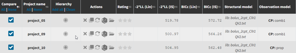
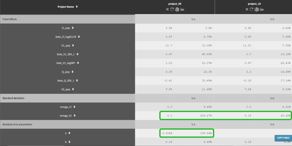
Until now, we have used the combined1 error model. The constant term “a” is estimated to be 0.027 in project_05, which is a little smaller than the smallest observation (around 0.1), and the RSE is estimated at 56%, meaning it is difficult to estimate. Thus it makes sense to try a model with a proportional error model only. We first create a project adding SEX as a covariate for both V1 and Q based on the covariate search, save it as project_09, and run it with the combined1 error model for comparison. The error model can be chosen in the “Statistical & Tasks” tab in the tab “Observation model” via the Error model drop down menu. We select proportional, save the project as project_10, and run the project.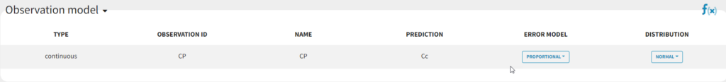
Convergence assessment
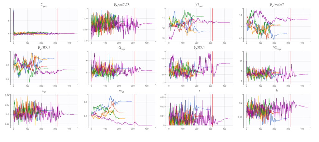
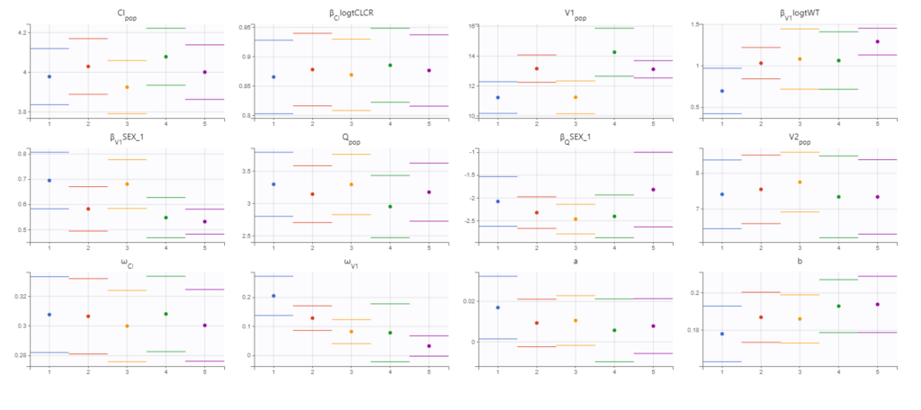
As a final check, we can do a convergence assessment, to verify that starting from different initial parameters or from different random number seeds leads to the same parameter estimates. Because Monolix will automatically generate ranges from which to sample the parameter bases on the initial estimates, we first click “Use last estimates: All” on the Initial estimates tab. Go back to Statistical model & Tasks and click on “Assessment” (below the run button), select 5 replicates with estimation of the standard errors and log-likelihood. To randomly pick initial values for all parameters, we select “All” under “sensitivity on initial parameters.” Monolix will automatically generate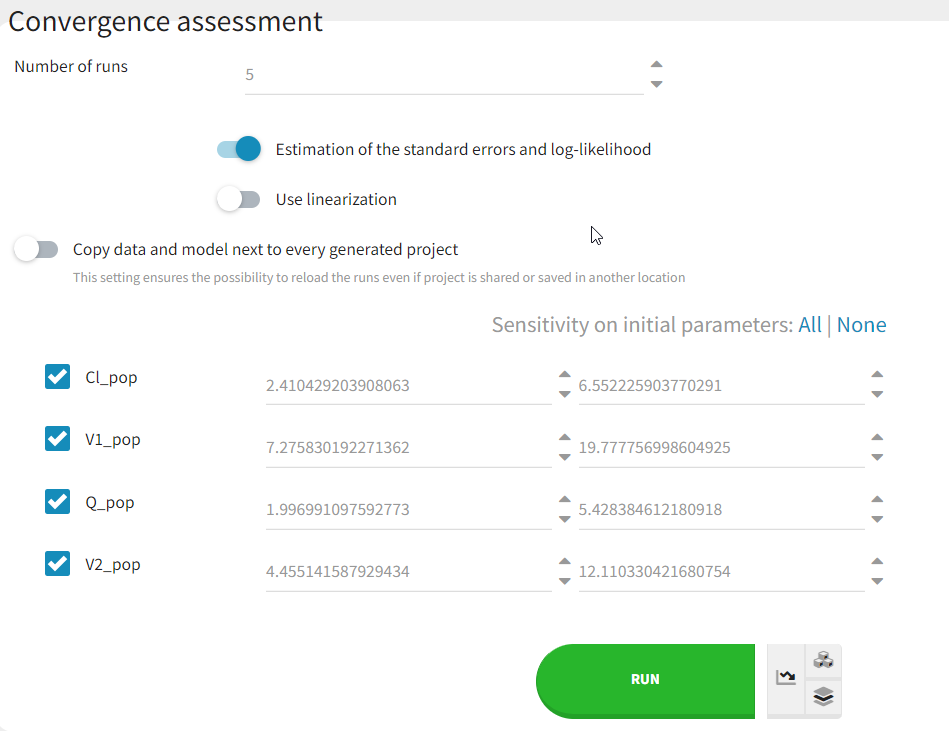
Final model summary
Our final model is the following:- 2-compartment model, parameterized as (Cl, V1, Q, V2)
- the residual error model is proportional
- Cl and V1have inter-individual variability, while Cl, V1, and Q have covariates. Their distributions for each parameter are:
$$Cl_i =Cl_{pop}\left(\frac{CLCR}{68}\right)^{\beta_{Cl,CLCR}} e^{\eta_{Cl,i}}$$
$$V1_i = V1_{pop}\left(\frac{WT}{70}\right)^{\beta_{V1,WT}} e^{\beta_{V1,SEX}1_{SEX_i=1}} e^{\eta_{V1,i}}$$
$$Q_i = Q_{pop} e^{\beta_{Q,SEX} 1_{SEX_i=1}} $$
$$V2_i = V2_{pop}$$
where 1_{SEX_i=1} is 1 if the SEX column has a value of 1 and 0 otherwise. Note that the SEX column is coded 0 or 1. The estimated parameters and their standard errors are: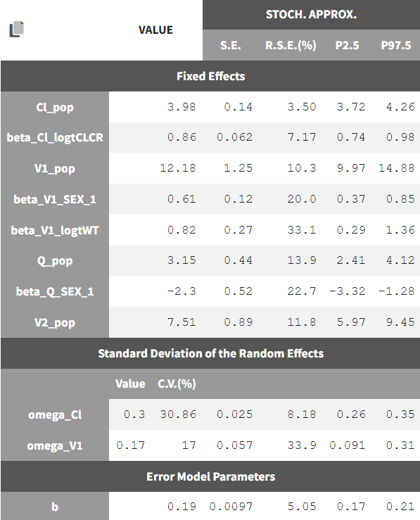
Click here to continue to Part 4: Simulations for individualized dosing with Simulx and Monolix