Tobramycin case study – Part 2: Exploratory Data Analysis

Download data set only | Monolix project files |  Simulx project files and scripts

[project files coming soon]

⚠️ Under construction ⚠️

This case study presents modeling of the tobramycin pharmacokinetics and determination of a priori dosing regimens in patients with various degrees of renal function impairment. It takes advantage of the integrated use of Monolix for data visualization and parameter estimation and Simulx for simulations and best dosing regimen determination. The case study is presented in 4 sequential parts which we recommend reading in order:

• Part 1: Introduction
• Part 2: Exploratory Data Analysis with Monolix
• Part 3: Model development with Monolix
• Part 4: Simulations for individualized dosing with Simulx and Monolix

Part 2: Exploratory data analysis with Monolix

Data set overview

Tobramycin bolus doses ranging from 20 to 140mg were administrated every 8 hours in 97 patients (45 females, 52 male) for 1 to 21 days (for most patients, for ~6 days).  Age, weight (kg), sex, height and creatinine clearance (mL/min) are available as covariates. Because height information was missing for around 30% of the patients, this covariate is ignored. The tobramycin concentration (mg/L) was measured 1 to 9 times per patients (322 measures in total), generally between 2 and 6h post-dose. Below is an extract of the data set file: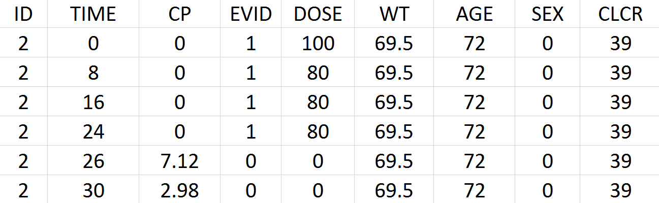

• ID: identifier of the patients
• TIME: time of dose or measurement (hours)
• CP: Tobramycin plasma concentration (mg/L)
• EVID: event identifier, 0=measurement, 1=dose
• DOSE: amount of the dose (mg)
• WT: weight (kg)
• AGE: age (years)
• SEX: 1=male, 0=female
• CLCR: creatinine clearance (mL/min)

Data set visualization with Monolix

We first start exploring the data set in Monolix. After having opened Monolix, we create a new project and load the data set. Based on the header, most columns are automatically recognized. 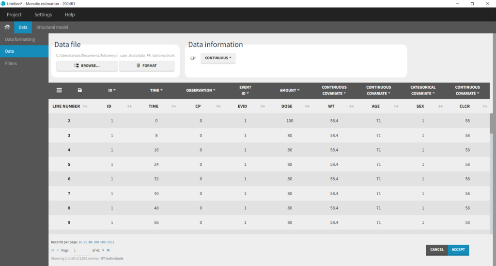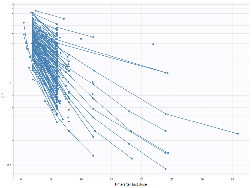The column-type must be set manually for the observed concentration (CP column set to column-type OBSERVATION), the dose (DOSE column set to column-type AMOUNT), and the creatinine clearance (CLCR column set to column-type CONTINUOUS COVARIATE for continuous covariate): After accepting the data mapping and clicking on the Plots tab, the spaghetti plot is displayed (figure below). It is possible to split or filter the plot using the covariates, which in the present case does not show any meaningful insights. To have a closer look at the elimination kinetic, we can examine only the last dose by setting the “Time after last dose” option for the x-axis and plotting the y-axis in log-scale. We observe the following kinetics. It is also interesting to display one covariate against another one. We, in particular, observe a negative correlation between age and creatinine clearance (correlation at -0.7): On the other hand, the creatinine clearance is similar for both sexes: In summary, from the exploratory data analysis, we have gained the following insights:

• A 1 compartment model with linear elimination is a good first approximation, and we can also explore a 2 compartment model.
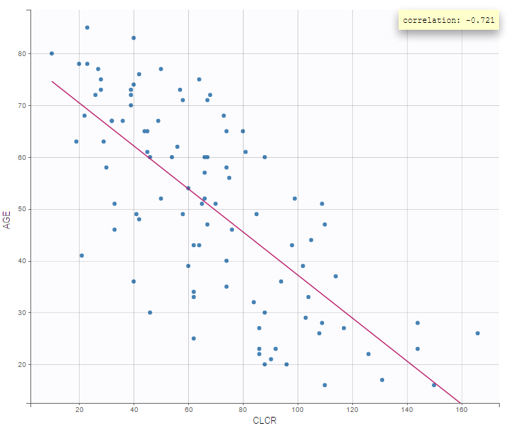
• Older patients have a lower creatinine clearance.

To continue to Part 3: Model development with Monolix, click here.